Team:TU Darmstadt/Modeling Docking
From 2012.igem.org
(→Results) |
(→Results) |
||
| Line 105: | Line 105: | ||
Here we illustrate the the docking results of TPF Fs. Cutinase: | Here we illustrate the the docking results of TPF Fs. Cutinase: | ||
| - | [[File: TPF.fsc.hist.png | | + | [[File: TPF.fsc.hist.png |900px|center]] |
Similar to the results of S-120, the active site residues are not identified under the best ranked docking results (accept for SER 120). | Similar to the results of S-120, the active site residues are not identified under the best ranked docking results (accept for SER 120). | ||
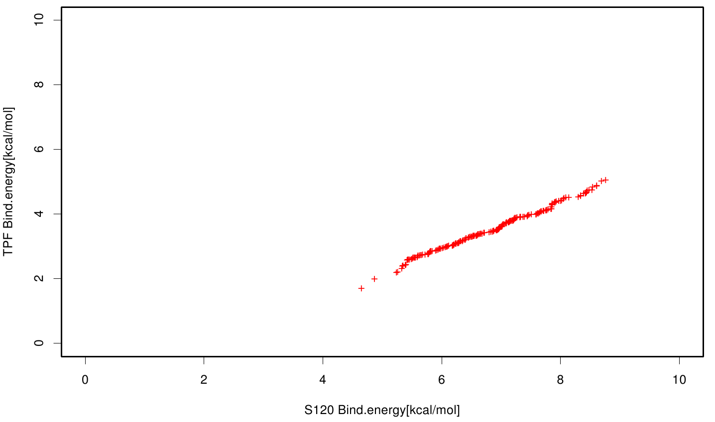
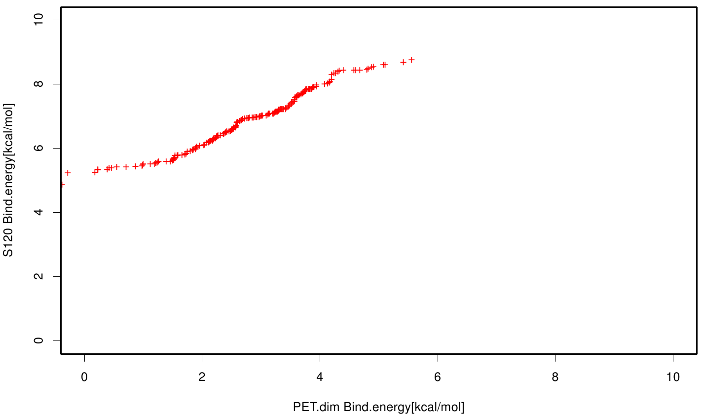
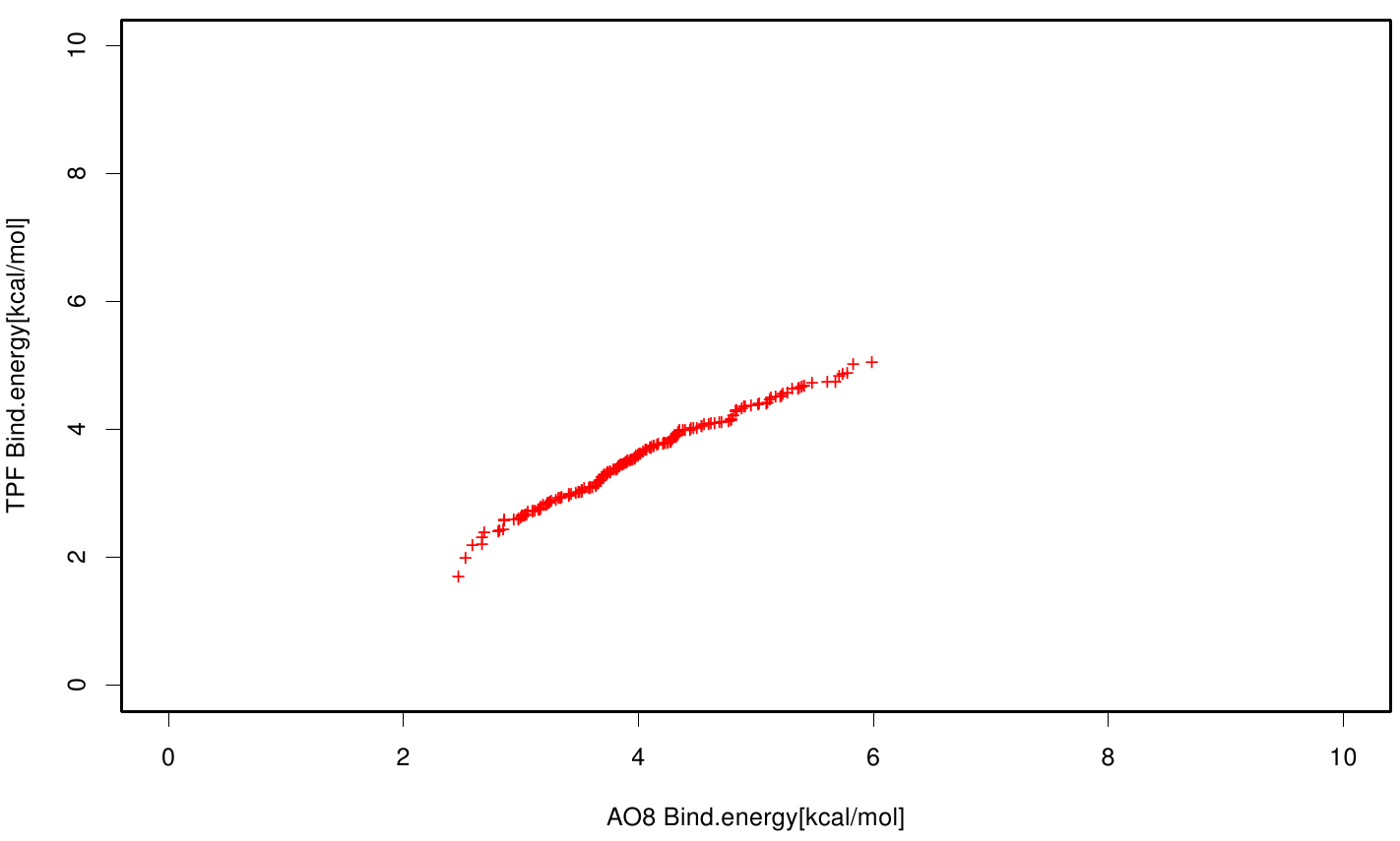
| + | The scatter plots of the binding constant are stored in the gallery below: | ||
| + | <gallery> | ||
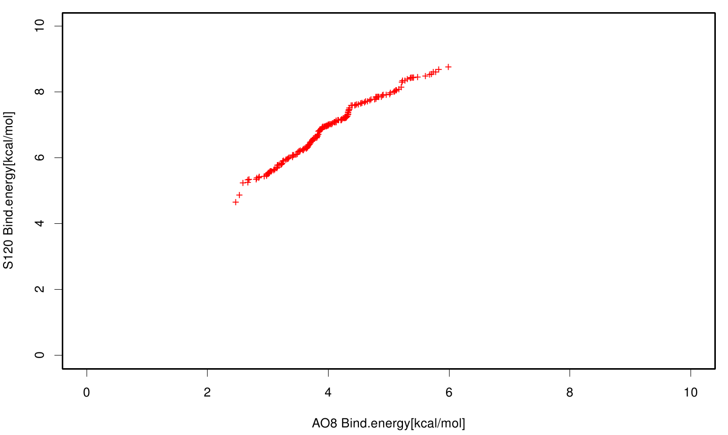
| + | File: AO8S120.fsc.scatter.bind.png | Scatter plot of AO8 vs. S120 | ||
| + | File: S120TPF.fsc.scatter.Bind.enery.png | Scatter plot of TPF vs. S120 | ||
| + | File: S120PET.fsc.scatter.bind.png | Scatter plot of PET vs. S120 | ||
| + | File: AO8TPF.fsc.scatter.bind.png | Scatter plot of AO8 vs. TPF | ||
| + | File: TPFPET.fsc.scatter.bind.png | Scatter plot of TPF vs. PET | ||
| + | File: AO8PET.fsc.scatter.bind.png | Scatter plot of AO8 vs. PET | ||
| + | </gallery> | ||
| + | |||
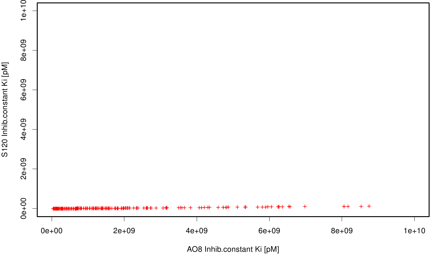
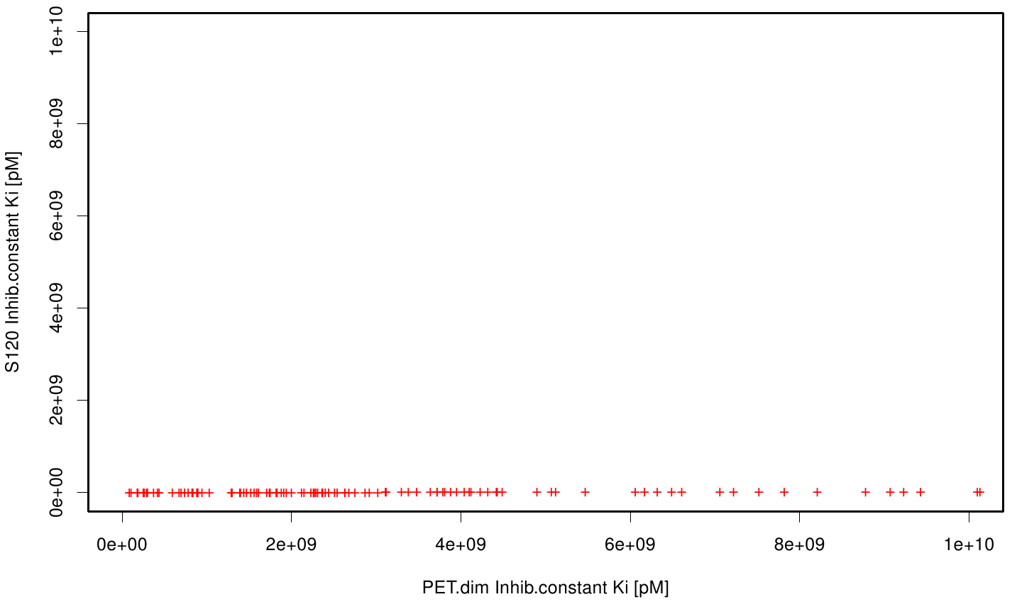
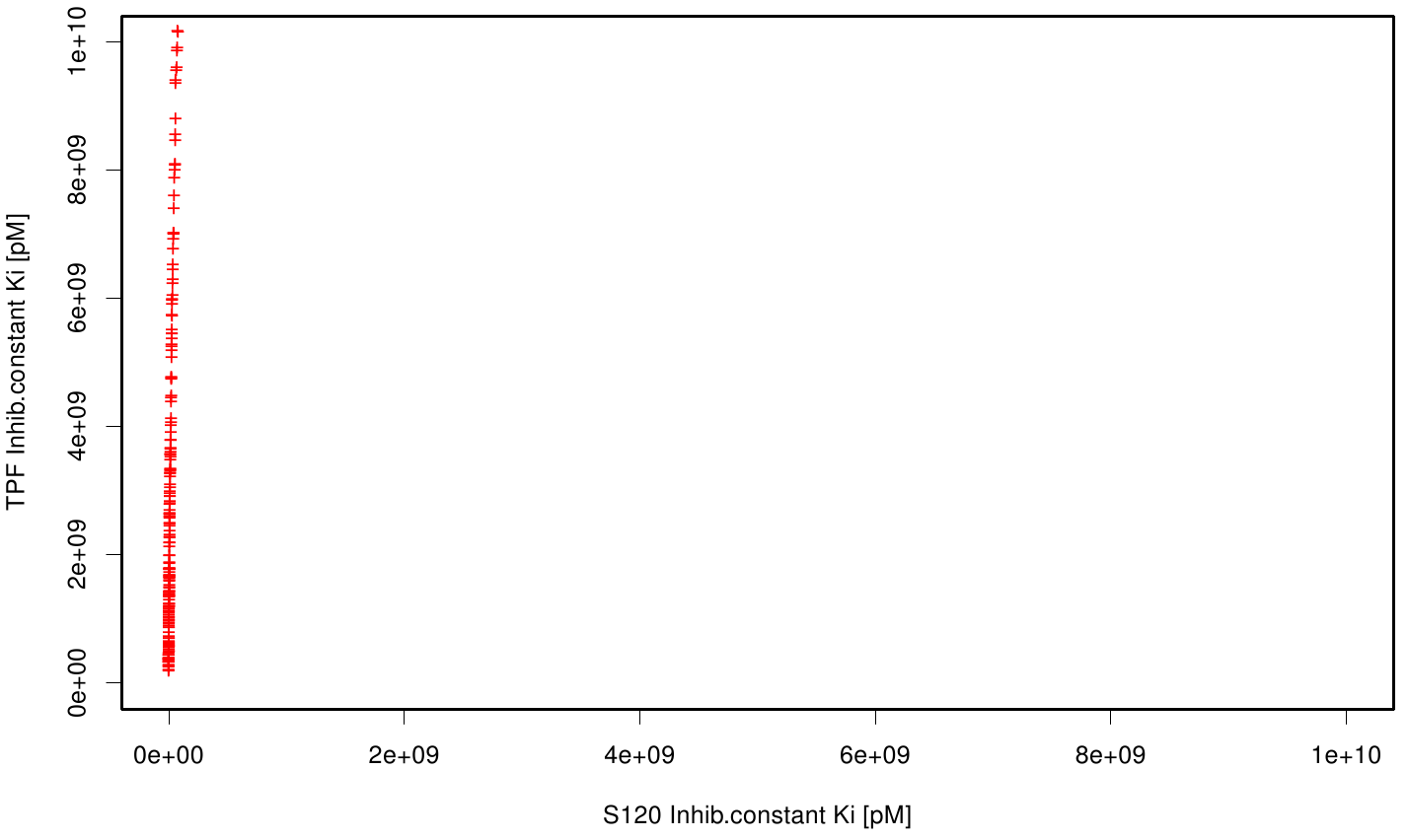
| + | The scatter plots of the inhibition constant are stored in the gallery below: | ||
| + | <gallery> | ||
| + | File: S120AO8.fsc.scatter.inhib.png | Scatter plot of AO8 vs. S120 | ||
| + | File: S120PET.fsc.scatter.inhib.png | Scatter plot of PET vs. S120 | ||
| + | File: S120TPF.fsc.scatter.inhib.png | Scatter plot of TPF vs. S120 | ||
| + | File: TPFPET.fsc.scatter.inhib.png | Scatter plot of TPF vs. PET | ||
| + | File: AO8PET.fsc.scatter.inhib.png | Scatter plot of AO8 vs. PET | ||
| + | File: AO8TPF.fsc.scatter.inhib.png | Scatter plot of AO8 vs. TPF | ||
| + | </gallery> | ||
Revision as of 17:09, 23 September 2012
| Homology Modeling | | Gaussian Networks | | Molecular Dynamics | | Information Theory | | Docking Simulation |
|---|
Contents |
Docking
Theory
Goal
While PET.er is degrading PET into its monomers various chemical compounds like polymer plasticizer are released. Since PET is itself a waste material, it will never be in a pure state. Due to this, it is important to study possible interaction of plasticizer as well as PET with the degradation machinery. Hence an experimental design will give a deeper understanding of the interaction of our enzymes with additives.
Methods
Due to the absence of forcefield terms of plasticizer we choose a global docking approach to study the interaction. For the docking simulations we uses the Autodock plugin of Yasara structure. Autodock is one of the ?? mreeost cized and scientific programs for Docking simulations. ??
Docking Protocol
For the docking approach we utilized the standard protocol dock_run.mcr and parallelized it up to six processors. Moreover, we choAse three additives out of the literature acting as the ligand within the simulations.
- OET-dimeric
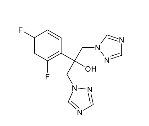
- S-120
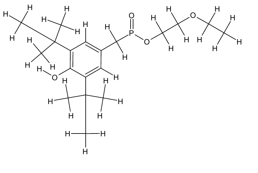
- AO-8
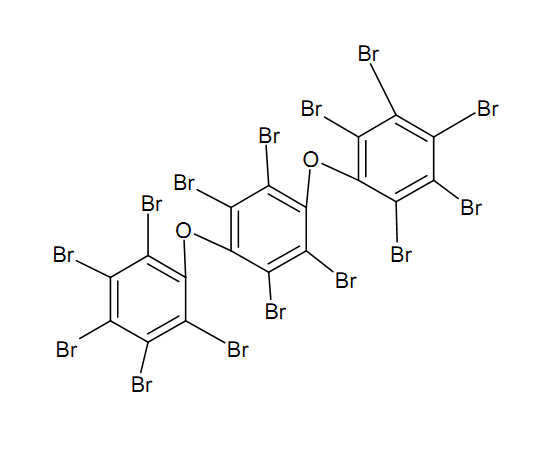
- TPF
Parameter for the Docking Experiment
- Ligands = S120, AO-8, TPF, dimer OET
- Receptors = PnB Esterase 13 (homology model) and Fs. Cutinase (PDB: 1CEX)
- Number of docking runs = 200
- ForceField AMBER03
- Flexible Ligand
Analytics
We extract binding energy from the atomic B-factors and the binding constant from the atomic property derived from all our calculations. We used scatter plots with the binding constant and the inhibition constant in order to compare the plasticizer as well as the PET substrate.We compared the binding energies as well as the inhibition constant from the best ranked docking runs.
Here, OET (dimeric state) became our reference substrate that means if an additive exhibit a higher inhibition constant it may effect our protein. Otherwise, if a binding energies exhibits a higher level than OET we can conclude that an additive may accumulate on our protein surface. Moreover, we compare the binding as well as the inhibition energies of the additives with itself to identify the strongest binder.
Hence we know the active site of the Fs. Cutinase and the PnB Est. 13 it will be interesting if a plastizicer may docks there. In order to analyze that, we counted the residues which are involved within every docking simulation. Therefore, we measured the distance of every ligand to its corresponding receptor with an appropriate threshold and thus identifying the residues.
Results
Interaction with Fs. Cutinase
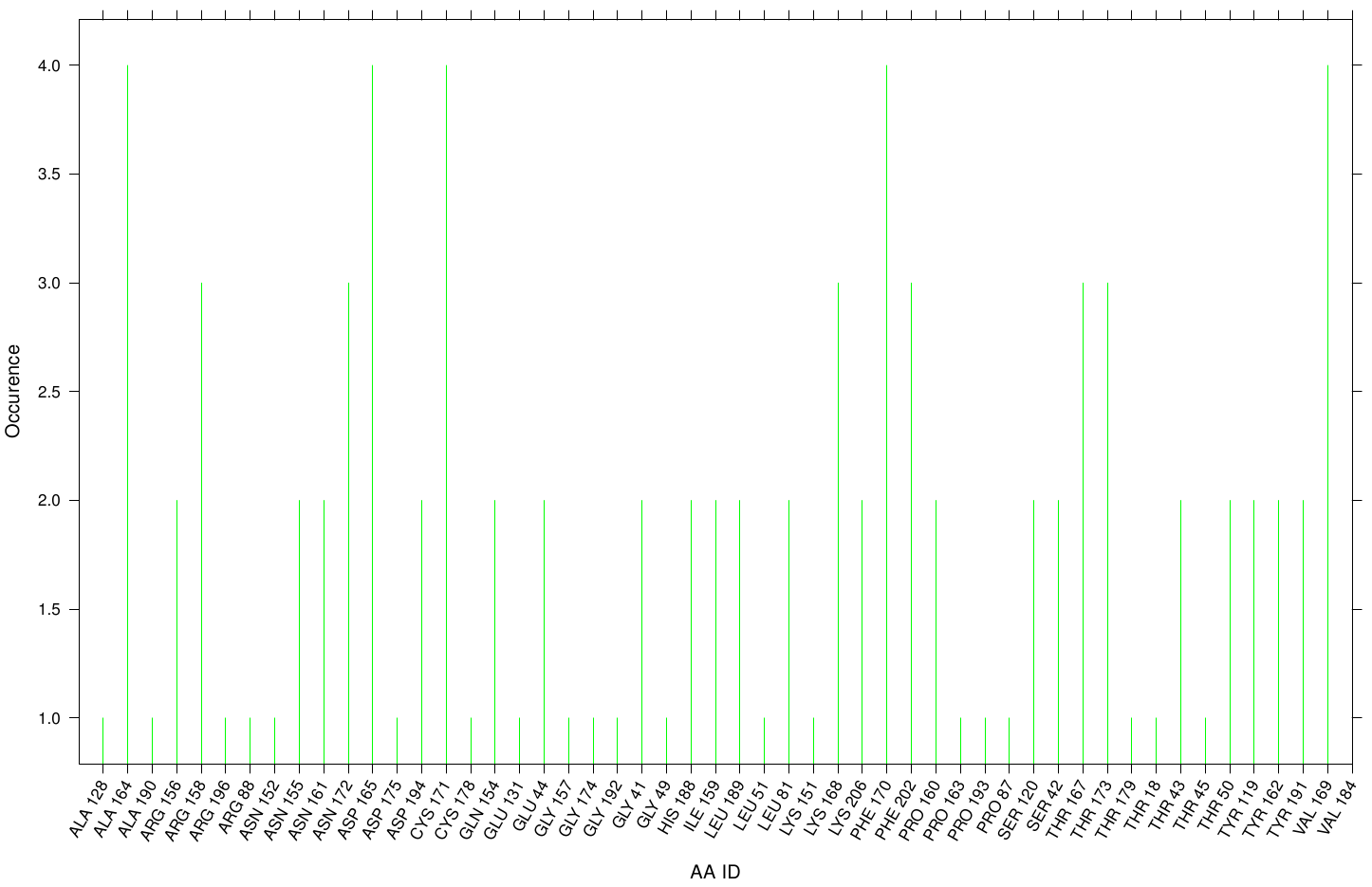
First we study the interaction of OET with the Fs. Cutinase. The following bar plot illustrate the occurrence of residues in direct contact with different ligand positions and conformations.
Within the best runs we got a wide range of involved residues. Since we we set no surface constrains, this is typically for a global docking approach.Here, the residues of the active site, ASP 165 (4 times), SER 120 (2 times) and HIS 188 (2 times), occurs under the best ranked runs. Interestingly, other hydrophobic residues like ALA 164 and VAL 169 are one of the high-scoring residues. Since these residues are located near the active site they may help to stabilize the PET Chains on top of the surface during the derogation process. Furthermore, it indicates that not only one time OET docked in the active site.
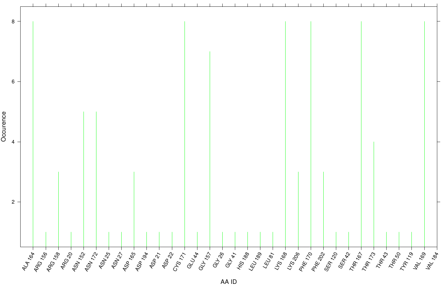
Here we illustrate the the docking results of S-120 with Fs. Cutinase:
Only a few residues are highly involved during the docking simulation. We can conclude that S-120 may not effect the active site. For this example we identified possible accumulation sites, CYS 171 LYS 206, and LYS 168 . Although, we didn't identified active site residues, we measured ALA 164 and VAL 169 as one of the high-scoring residues.
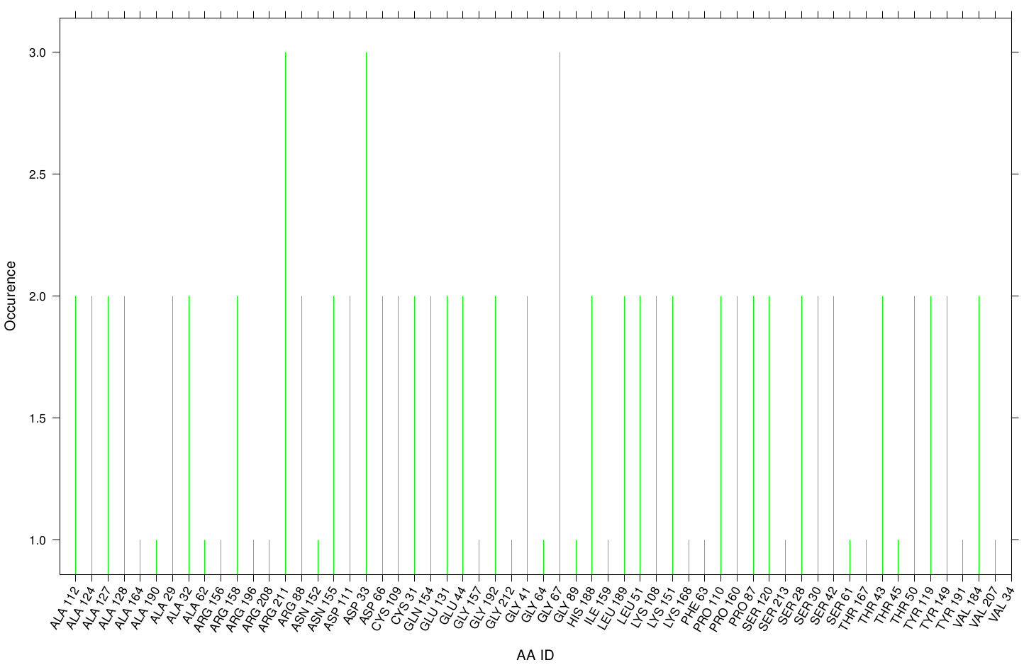
Here we illustrate the the docking results of AO-8 with Fs. Cutinase:
Interestingly, we can observe nearly a uniform distribution of residue occurrence. Due to the hydrophobic nature of AO-8 it is obvious that it distribute ubiquity over the surface.
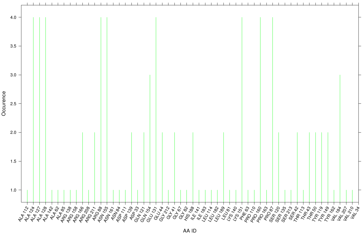
Here we illustrate the the docking results of TPF Fs. Cutinase:
Similar to the results of S-120, the active site residues are not identified under the best ranked docking results (accept for SER 120). The scatter plots of the binding constant are stored in the gallery below:
The scatter plots of the inhibition constant are stored in the gallery below:
 "
"

