"
"
Team:KAIST Korea/Project Modeling
From 2012.igem.org
(Difference between revisions)
| Line 184: | Line 184: | ||
</div> | </div> | ||
</br> | </br> | ||
| - | <span id='little'>We also consider concentration of GFP/RFP of cell colony. The solution curve shown below represents that result.</span> | + | <span id='little'>We also consider concentration of GFP/RFP of cell colony. The solution curve shown below represents that result.</span></br> |
<div align="center" ><img src='https://static.igem.org/mediawiki/2012/b/b8/KAIST_Result_graph_gfprfp2.png'/></div> | <div align="center" ><img src='https://static.igem.org/mediawiki/2012/b/b8/KAIST_Result_graph_gfprfp2.png'/></div> | ||
</section> | </section> | ||
| - | + | </br> | |
<div align='right'><a href="#top">▲ Back to the top</a></div></br></br> | <div align='right'><a href="#top">▲ Back to the top</a></div></br></br> | ||
<div> | <div> | ||
| Line 196: | Line 196: | ||
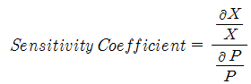
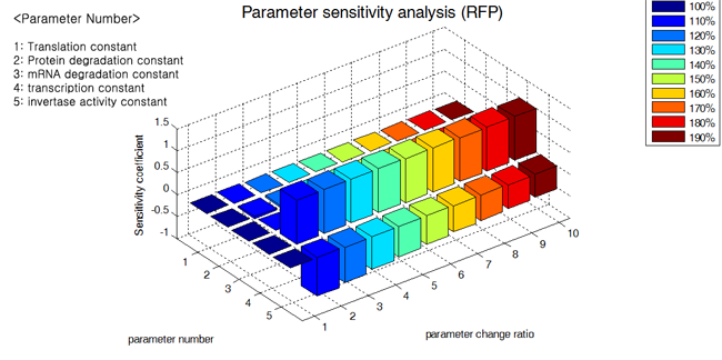
<span id="little">We also do parameter sensitivity analysis to find what kind of parameters are critically impact on our system. We define sensitivity coefficient and calculate as paramters vary with some ratio. </span></br></br> | <span id="little">We also do parameter sensitivity analysis to find what kind of parameters are critically impact on our system. We define sensitivity coefficient and calculate as paramters vary with some ratio. </span></br></br> | ||
<div align="center" ><img src='https://static.igem.org/mediawiki/2012/d/d3/KAIST_Sensitivity_coeff.png'/></div></br> | <div align="center" ><img src='https://static.igem.org/mediawiki/2012/d/d3/KAIST_Sensitivity_coeff.png'/></div></br> | ||
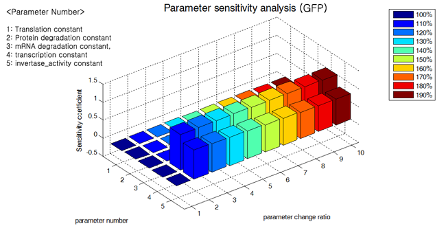
| - | <span id="little">And We plot the result using 3d bar graph. As graph represents, some parameters are critical to change the output of our system and some are not.</span> | + | <span id="little">And We plot the result using 3d bar graph. As graph represents, some parameters are critical to change the output of our system and some are not.</span></br></br> |
| - | <div align="center" ><img src='https://static.igem.org/mediawiki/2012/1/1d/KAIST_Sensitivityresult.png'/></div | + | <div align="center" ><img src='https://static.igem.org/mediawiki/2012/1/1d/KAIST_Sensitivityresult.png'/></div></br> |
| - | <div align="center" ><img src='https://static.igem.org/mediawiki/2012/c/c8/Sensitivityresult2.png'/></div | + | <div align="center" ><img src='https://static.igem.org/mediawiki/2012/c/c8/Sensitivityresult2.png'/></div> |
| Line 211: | Line 211: | ||
</ul> | </ul> | ||
</br> | </br> | ||
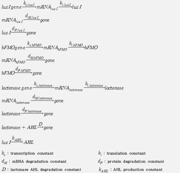
| - | <span id="little">Similar to ' | + | <span id="little">Similar to 'Proof of concept, mathematical model', we can write simplified equation of our system, that is shown below.</span></br></br> |
| - | <div align="center" ><img src='https://static.igem.org/mediawiki/2012/thumb/1/1b/KAIST_ReactionofbFMO.png/623px-KAIST_ReactionofbFMO.png'/></div></br></br> | + | <div align="center" ><img src='https://static.igem.org/mediawiki/2012/thumb/1/1b/KAIST_ReactionofbFMO.png/623px-KAIST_ReactionofbFMO.png'/></div></br> |
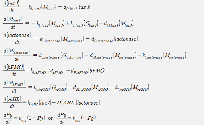
| - | + | <span id='little'>Based on above reaction, we construct our mathematical model like this.</span></br></br> | |
| + | <div align="center" ><img src='https://static.igem.org/mediawiki/2012/e/ed/KAIST_ODEbFMO.png'/></div></br> | ||
| + | <span id='little'>Using MATLAB we can solve these set of differential equations and get solution curve like below.</span></br></br> | ||
| + | <div align="center" ><img src='https://static.igem.org/mediawiki/2012/8/8e/KAIST_Result_graph_bFMO1.png'/></div></br> | ||
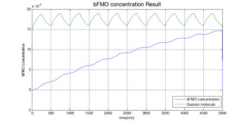
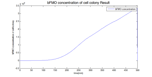
| + | <span id='little'>When we consider the cell colony instead of one cell, we simply multiply cell growth curve to original result. And derived curve is like below.</span></br></br> | ||
| + | <div align="center" ><img src='https://static.igem.org/mediawiki/2012/7/77/KAIST_Result_graph_bFMO2.png'/></div></br> | ||
</div> | </div> | ||
| + | </section> | ||
| + | </br> | ||
| + | <div align='right'><a href="#top">▲ Back to the top</a></div></br></br> | ||
| + | <div> | ||
| + | <ul><li style="list-style-type:square;font-size:14px;font-weight:bold;">Parameter Sensitivity Analysis</li></ul> | ||
| + | </br> | ||
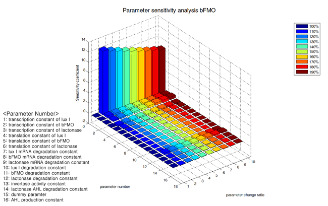
| + | <span id='little'>We also do parameter sensitivity analysis and result is like below.</span> | ||
| + | <div align="center" ><img src='https://static.igem.org/mediawiki/2012/6/60/KAIST_sensitivityresult3.png'/></div></br> | ||
| + | </div> | ||
| + | </br></br> | ||
| + | <div align='right'><a href="#top">▲ Back to the top</a></div></br></br> | ||
| + | |||
</div> | </div> | ||
</div> | </div> | ||
Revision as of 17:27, 26 October 2012


2012 KAIST Korea
Mail : kaist.igem.2012@gmail.com
Twitter : twitter.com/KAIST_iGEM_2012
Facebook : www.facebook.com/KAISTiGEM2012


Project : Modeling

Cell Growth Curve
Proof of concept
Auto Regulation

 And We plot the result using 3d bar graph. As graph represents, some parameters are critical to change the output of our system and some are not.
Modeling
Computational modeling of our project
Cell Growth Curve
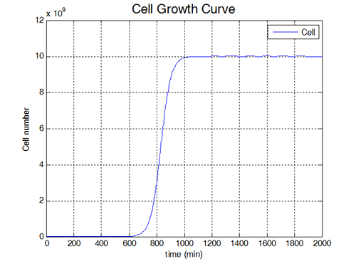
Cell growth can be modeled using Logistic differential equation as shown below.
 When we solve this equation with appropriate parameters(using MATLAB), we can get solution curve as shown below. This curve matches with our knowledge about cell growth.
Proof of concept
 Using these reaction, we constructed mathematical model of our system as shown below. Pg(gene probability), in our model, represents the number of plasmid which is inverted. And the rate of producing inverted gene is reduced as the remaining non-inverted gene is reduced.
 Using MATLAB we can solve these set of differential equations and get solution curve like below.
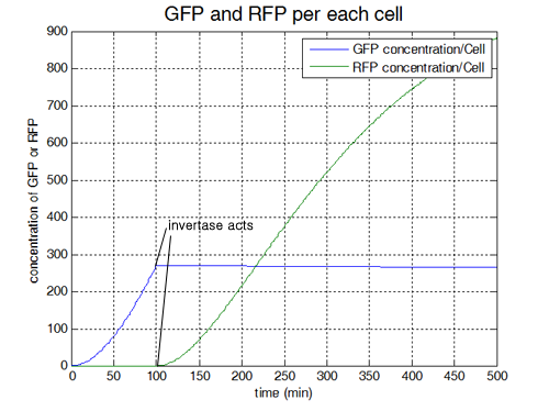
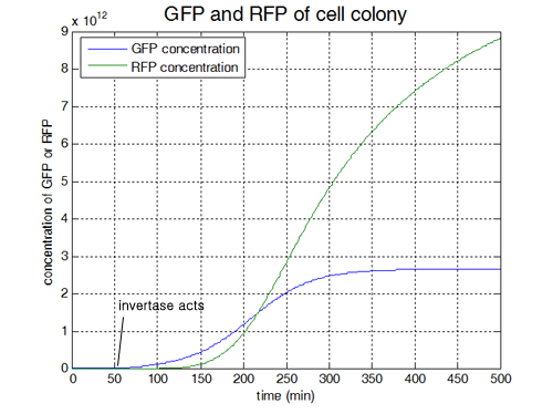
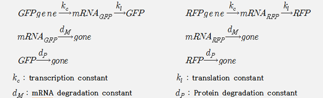
We also consider concentration of GFP/RFP of cell colony. The solution curve shown below represents that result.
- Mathematical model
- Parameter Sensitivity Analysis
Auto Regulation
 Based on above reaction, we construct our mathematical model like this.
 Using MATLAB we can solve these set of differential equations and get solution curve like below.
 When we consider the cell colony instead of one cell, we simply multiply cell growth curve to original result. And derived curve is like below.
- Mathematical model
- Parameter Sensitivity Analysis