"
"
Team:Cornell/project/drylab/modeling/time response
From 2012.igem.org
(Difference between revisions)
(Created page with "{{:Team:Cornell/templates/header}} <!-- paulirish.com/2008/conditional-stylesheets-vs-css-hacks-answer-neither/ --> <!--[if lt IE 7]> <html class="no-js lt-ie9 lt-ie8 lt-ie7" lan...") |
|||
| (76 intermediate revisions not shown) | |||
| Line 7: | Line 7: | ||
<!--<![endif]--> | <!--<![endif]--> | ||
| - | <script type="text/x-mathjax-config"> | + | <script type="text/x-mathjax-config"> |
| - | + | MathJax.Hub.Config({tex2jax: {inlineMath: [['$','$'], ['\\(','\\)']]}}); | |
| - | </script> | + | </script> |
| - | <script type="text/javascript" | + | <script type="text/javascript" |
| - | + | src="http://cdn.mathjax.org/mathjax/latest/MathJax.js?config=TeX-AMS-MML_HTMLorMML"></script> | |
| - | </script> | + | |
| - | + | ||
<div class="row"> | <div class="row"> | ||
| Line 23: | Line 21: | ||
<li class="divider"></li> | <li class="divider"></li> | ||
<li> | <li> | ||
| - | + | <a href="https://2012.igem.org/Team:Cornell/project/drylab">How It Works</a> | |
| - | + | </li> | |
| - | + | <li> | |
| - | + | <a href="https://2012.igem.org/Team:Cornell/project/drylab/functional_requirements">Functional Requirements</a> | |
| - | + | </li> | |
| - | + | <li> | |
| - | + | <a href="https://2012.igem.org/Team:Cornell/project/drylab/components">Components</a> | |
| - | + | </li> | |
| - | <li> Modeling | + | <li> |
| - | <ul> | + | Modeling |
| + | <ul> | ||
<li> | <li> | ||
<a href="https://2012.igem.org/Team:Cornell/project/drylab/modeling/deployment">Deployment</a> | <a href="https://2012.igem.org/Team:Cornell/project/drylab/modeling/deployment">Deployment</a> | ||
| - | </li | + | </li> |
| - | <li> | + | <li class ="active"> |
<a href="https://2012.igem.org/Team:Cornell/project/drylab/modeling/time_response">Time Response</a> | <a href="https://2012.igem.org/Team:Cornell/project/drylab/modeling/time_response">Time Response</a> | ||
</li> | </li> | ||
| - | </ | + | </ul> |
| - | </ | + | </li> |
| - | + | <li> | |
| - | + | <a href="https://2012.igem.org/Team:Cornell/project/drylab/status">Device Status</a> | |
| - | + | </li> | |
| - | + | ||
</ul> | </ul> | ||
</div> | </div> | ||
| Line 57: | Line 56: | ||
<div class="nine columns"> | <div class="nine columns"> | ||
| - | <h3> | + | <h3>How do our sensors respond to varying analyte concentration over time?</h3> |
| + | |||
| + | To make sense of data collected remotely, we must know the time it takes for our sensor to produce a signal in response to a change in analyte concentration in the sample stream. In other words, we need to know whether current output at any time can be taken to represent analyte concentration <i> at that time </i>, or whether our system has memory. From preliminary data presented for our arsenic sensor in our <a href="https://2012.igem.org/Team:Cornell/project/wetlab/results/currentresponse"> results page</a>, we know the response time of the S.A.F.E. B.E.T. sensor is on the order of 1.5 days. That is, it takes nearly a day and a half for our system to fully respond upon a sudden change in analyte concentration in the reactor. | ||
| + | <br> | ||
| + | <br> | ||
| + | However, knowledge of the characteristic response time is insufficient to predict the dynamic behavior of our sensor when the concentration of analyte is variable in time. In other words, the response time of the sensor can tell us how long it takes our system to respond to a single perturbation in analyte concentration, but further analysis is necessary in the prediction of the sensor’s response to continuously changing analyte concentration. For example, if changes in concentration occur slowly over time, our sensor may produce a signal that perfectly tracks the analyte concentration—with some lag. On the other hand, if changes occur quickly in relation to the response time of the sensor, we might expect an output corresponding to a time-average of the analyte concentration. Here, we model the current output of our sensor in response to oscillating concentration of analyte in order to predict the time-scales over which the S.A.F.E. B.E.T. sensor filters out fine changes in analyte concentration. | ||
| - | |||
</div> | </div> | ||
<div class="three columns"> | <div class="three columns"> | ||
| - | <img src="https://static.igem.org/mediawiki/2012/ | + | <img src="https://static.igem.org/mediawiki/2012/a/a7/Cornell_TR_River.jpg"> |
</div> | </div> | ||
</div> | </div> | ||
<div class="row" id="item2"> | <div class="row" id="item2"> | ||
| - | <div class=" | + | <div class="four columns" style="text-align:center;"> |
| - | <img src="https://static.igem.org/mediawiki/2012/ | + | <a href="https://static.igem.org/mediawiki/2012/6/6e/Cornell_RT_Reactor.png" rel="lightbox"> <img class="inline" src="https://static.igem.org/mediawiki/2012/2/2f/Cornell_RT_Reactor_SQ.png">Click to Enlarge</a> |
| + | |||
</div> | </div> | ||
| - | <div class=" | + | <div class="eight columns"> |
| - | <h3> | + | <h3>Problem Setup</h3> |
| - | + | As seen in the figure to the left, the S.A.F.E. B.E.T. sensor is a continuous flow reactor, with the feed rate at the inlet equal to the effluent flow rate—at a value of $F$ = 18 mL/min. The reactor has constant volume of 120 mL. | |
| + | <br><br> | ||
| + | We want to know how our system responds to oscillating analyte concentration in the feed stream—<i>i.e.</i>, the river in which the sensor is deployed. To this end, we will model time varying analyte concentration $([A](t))$ as a sine wave. The frequency of this wave will be the parameter of primary interest, since we are particularly interested in determining the timescales over which the S.A.F.E. B.E.T. sensor produces a signal that tracks fine changes in analyte concentration. | ||
| + | <br><br> | ||
| + | However, before we can determine our sensor's current response to an input function of varying river analyte concentration, we must first solve for the concentration of analyte <i>in the reactor</i> as a function of time $(c(t))$. Therefore, our solution will consist of two coupled differential equations—one which may be solved analytically for $c(t)$ and one which may be numerically solved for the current response of the S.A.F.E. B.E.T. sensor—as described below. | ||
| - | |||
| - | + | </div> | |
| - | + | </div> | |
| - | + | <div class="row" id="item3"> | |
| + | <div class="nine columns"> | ||
| - | $$ | + | <h3>Solution</h3> |
| + | <h5>Concentration of Analyte In Reactor</h5> | ||
| + | First, we need to solve for the concentration of analyte in the reactor as a function of time $(c(t))$ given an oscillating input of analyte $([A](t))$—with arbitrary frequency and amplitude—in the river. By performing a mass balance around the reactor (and ignoring any contribution from generation or consumption), we may write the following differential equation: | ||
| - | + | $$\frac{dc}{dt} = [A](t)\cdot\frac{F}{V}-c\cdot\frac{F}{V}=D([A](t)-c),$$ | |
| - | $$ | + | $$ \mathrm{where} \ \ [A](t) = A_0\cdot\sin(2 \pi ft)+A_0,$$ |
| + | and the dilution rate, $D$, equals 3.6 day$^{-1}$ for our system. Using $e^{Dt}$ as an integrating factor, we find | ||
| - | + | $$c(t) = \frac{(A0 (D^2 \sin(2 \pi f t)+D^2-2 \pi D f \cos(2 \pi f t)+4 \pi^2 f^2))}{(D^2+4 \pi^2 f^2)}+k_1 e^{-D t}$$ | |
| - | $$ | + | $$ \mathrm{where} \ \ k_1 = - \frac{(A_0 (D^2-2 \pi D f+4 \pi^2))}{(D^2+4 \pi^2 f^2)} \ \ \mathrm{such\ that} \ c(0) =0 $$ |
| - | + | <br> | |
| + | <br> | ||
| + | <h5>Current Response</h5> | ||
| + | Now that we have an analytical solution for the concentration of analyte in the reactor over time, we wish to model the current response given the input function $c(t)$. To accomplish this, we model the time rate of change of current of our arsenic sensor using a Hill function [1] with a cooperativity coefficient of unity—fitting data presented in Fig. 3 of our <a href="https://2012.igem.org/Team:Cornell/project/wetlab/results/currentresponse">Current Response </a>characterization page—and lumping all transcriptional, translational, and post-translational processes: | ||
| - | $$ | + | $$\frac{dI}{dt} = \frac{\beta_1 \cdot c(t)}{c_{1/2}+c(t)}+\beta_0 - \alpha I, $$ |
| - | + | where $c(t)$ is as defined above; $\beta_1$ is 1.4 $\mu$A/day, $\beta_0$ is 2.8 $\mu$A/day, $c_{1/2}$, the half-saturating analyte concentration, is 100 $\mu$M, $\alpha$ = 0.69 day$^{-1}$; and the saturating current output is $(\beta_1 + \beta_0)/\alpha$. | |
| + | <br> | ||
| + | <br> | ||
| + | Using this ordinary differential equation, we may numerically solve for current as a function of time—given the input function derived above. The results of such numerical solutions for input functions with various frequencies—<a href="https://static.igem.org/mediawiki/2012/6/67/ShewieTime.m" target="_blank">performed </a>using the differential equation solver ode45 in MATLAB—are shown below. | ||
| - | + | </div> | |
| - | + | <div class="three columns"> | |
| + | <img src="https://static.igem.org/mediawiki/2012/d/d0/Cornell_mathhhh.jpg"> | ||
| + | </div> | ||
| + | </div> | ||
| + | |||
| + | <div class="row" id="item4"> | ||
| + | <div class="three columns"> | ||
| + | <img src="https://static.igem.org/mediawiki/2012/0/07/Cornell_MATLAB.png"> | ||
| + | </div> | ||
| + | <div class="nine columns"> | ||
| + | <h3>Results: Time-Averaged Output for Rapidly Oscillating Analyte Concentrations</h3> | ||
| + | As seen below in Fig. 1, variations in analyte concentration on the order of 90 days can be detected by the S.A.F.E. B.E.T. sensor without time-averaging. In other words, the signal produced by the sensor tracks the changes in analyte without disruption from the ‘memory’ of the system. This is important, since we know our sensor can reliably report analyte concentration at any given time once we account for the simple time lag of the response time—which is negligible for variations on timescales of weeks or greater. | ||
| + | <br><br> | ||
| + | <img class="inline" src="https://static.igem.org/mediawiki/2012/a/a7/Cornell_TR1.png"> | ||
| + | <h6>Fig. 1. A sinusoidally oscillating concentration of analyte (with period, T, of 90 days) in the feed stream (green) is plotted alongside the modeled sensor output (blue). For analyte changes on this timescale, current output traverses the entire range of the outputs from basal current of 4 $\mu$A to saturating current just under 6 $\mu$A— giving a fine-tuned output corresponding to analyte concentrations within the dynamic range. </h6> | ||
| + | |||
| + | <br> | ||
| + | <br><br> | ||
| + | However, for variations in analyte that occur on timescales of less than a month, the ‘memory’ of the system begins to interfere with our sensor’s ability to track fine changes in analyte concentration. As seen in Fig. 2 below, when oscillations in analyte concentration occur on the order of days, the response of our sensor approaches a constant output that accurately represents the time-average of the oscillating analyte concentration. Even though S.A.F.E. B.E.T. cannot track fine changes on these timescales, the ability to sense the time-averaged value represents a significant improvement over current detection methods that rely on ‘spot’ sampling—which often misrepresents the true analyte concentration. | ||
| + | <br><br> | ||
| + | |||
| + | <img class="inline" src="https://static.igem.org/mediawiki/2012/2/29/Cornell_TR2.png"> | ||
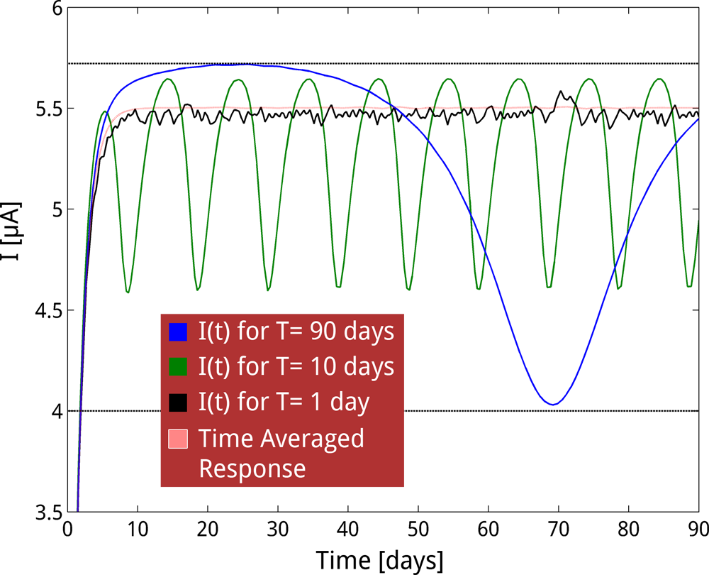
| + | <h6>Fig. 2. Modeled current output of the S.A.F.E. B.E.T. sensor is plotted as a function of time for input functions corresponding to varying river analyte concentrations—with oscillatory periods of 90 days (blue), 10 days (green) and 1 day (black). As in Fig. 1, for analyte changes on the order of 90 days, the sensor produces a fine-tuned output corresponding to analyte concentrations within its dynamic range. As the frequency of analyte variation increases, the current response approaches that expected from the time-averaged concentration (pink dash). </h6> | ||
</div> | </div> | ||
| Line 105: | Line 144: | ||
</div> | </div> | ||
| - | |||
| - | |||
| - | |||
<div class="row last-ele"> | <div class="row last-ele"> | ||
<div class="twelve columns"> | <div class="twelve columns"> | ||
<h3>References</h3> | <h3>References</h3> | ||
| - | [1] | + | [1] Hill, A. (1910) The possible effects of the aggregation of the molecules of haemoglobin on its dissociation curves. J Physiol 40: 4–7. |
| - | + | ||
| - | + | ||
| - | + | ||
| - | + | ||
</div> | </div> | ||
</div> | </div> | ||
| - | |||
| - | |||
| - | |||
| - | |||
</div> | </div> | ||
| Line 129: | Line 157: | ||
<script src="https://2012.igem.org/Team:Cornell/javascripts/foundation.min?action=raw&ctype=text/javascript"></script> | <script src="https://2012.igem.org/Team:Cornell/javascripts/foundation.min?action=raw&ctype=text/javascript"></script> | ||
<script src="https://2012.igem.org/Team:Cornell/javascripts/app?action=raw&ctype=text/javascript"></script> | <script src="https://2012.igem.org/Team:Cornell/javascripts/app?action=raw&ctype=text/javascript"></script> | ||
| + | <script src="https://2012.igem.org/Team:Cornell/javascripts/lightbox?action=raw&ctype=text/javascript"></script> | ||
<script type="text/javascript"> | <script type="text/javascript"> | ||
$(window).load(function() { | $(window).load(function() { | ||
Latest revision as of 07:35, 10 November 2012


-
Dry Lab
- How It Works
- Functional Requirements
- Components
- Modeling
- Device Status
Time Response
How do our sensors respond to varying analyte concentration over time?
To make sense of data collected remotely, we must know the time it takes for our sensor to produce a signal in response to a change in analyte concentration in the sample stream. In other words, we need to know whether current output at any time can be taken to represent analyte concentration at that time , or whether our system has memory. From preliminary data presented for our arsenic sensor in our results page, we know the response time of the S.A.F.E. B.E.T. sensor is on the order of 1.5 days. That is, it takes nearly a day and a half for our system to fully respond upon a sudden change in analyte concentration in the reactor.However, knowledge of the characteristic response time is insufficient to predict the dynamic behavior of our sensor when the concentration of analyte is variable in time. In other words, the response time of the sensor can tell us how long it takes our system to respond to a single perturbation in analyte concentration, but further analysis is necessary in the prediction of the sensor’s response to continuously changing analyte concentration. For example, if changes in concentration occur slowly over time, our sensor may produce a signal that perfectly tracks the analyte concentration—with some lag. On the other hand, if changes occur quickly in relation to the response time of the sensor, we might expect an output corresponding to a time-average of the analyte concentration. Here, we model the current output of our sensor in response to oscillating concentration of analyte in order to predict the time-scales over which the S.A.F.E. B.E.T. sensor filters out fine changes in analyte concentration.

 Click to Enlarge
Problem Setup
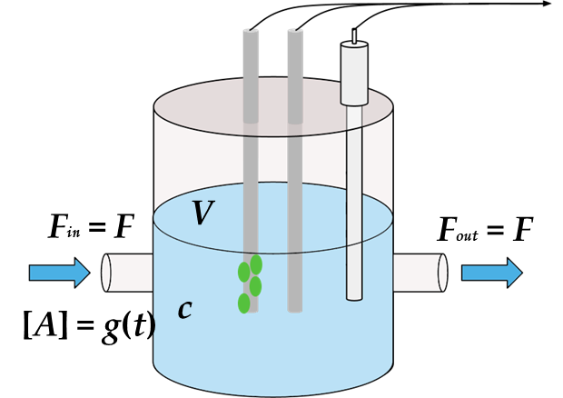
As seen in the figure to the left, the S.A.F.E. B.E.T. sensor is a continuous flow reactor, with the feed rate at the inlet equal to the effluent flow rate—at a value of $F$ = 18 mL/min. The reactor has constant volume of 120 mL.We want to know how our system responds to oscillating analyte concentration in the feed stream—i.e., the river in which the sensor is deployed. To this end, we will model time varying analyte concentration $([A](t))$ as a sine wave. The frequency of this wave will be the parameter of primary interest, since we are particularly interested in determining the timescales over which the S.A.F.E. B.E.T. sensor produces a signal that tracks fine changes in analyte concentration.
However, before we can determine our sensor's current response to an input function of varying river analyte concentration, we must first solve for the concentration of analyte in the reactor as a function of time $(c(t))$. Therefore, our solution will consist of two coupled differential equations—one which may be solved analytically for $c(t)$ and one which may be numerically solved for the current response of the S.A.F.E. B.E.T. sensor—as described below.
Solution
Concentration of Analyte In Reactor
First, we need to solve for the concentration of analyte in the reactor as a function of time $(c(t))$ given an oscillating input of analyte $([A](t))$—with arbitrary frequency and amplitude—in the river. By performing a mass balance around the reactor (and ignoring any contribution from generation or consumption), we may write the following differential equation: $$\frac{dc}{dt} = [A](t)\cdot\frac{F}{V}-c\cdot\frac{F}{V}=D([A](t)-c),$$ $$ \mathrm{where} \ \ [A](t) = A_0\cdot\sin(2 \pi ft)+A_0,$$ and the dilution rate, $D$, equals 3.6 day$^{-1}$ for our system. Using $e^{Dt}$ as an integrating factor, we find $$c(t) = \frac{(A0 (D^2 \sin(2 \pi f t)+D^2-2 \pi D f \cos(2 \pi f t)+4 \pi^2 f^2))}{(D^2+4 \pi^2 f^2)}+k_1 e^{-D t}$$ $$ \mathrm{where} \ \ k_1 = - \frac{(A_0 (D^2-2 \pi D f+4 \pi^2))}{(D^2+4 \pi^2 f^2)} \ \ \mathrm{such\ that} \ c(0) =0 $$Current Response
Now that we have an analytical solution for the concentration of analyte in the reactor over time, we wish to model the current response given the input function $c(t)$. To accomplish this, we model the time rate of change of current of our arsenic sensor using a Hill function [1] with a cooperativity coefficient of unity—fitting data presented in Fig. 3 of our Current Response characterization page—and lumping all transcriptional, translational, and post-translational processes: $$\frac{dI}{dt} = \frac{\beta_1 \cdot c(t)}{c_{1/2}+c(t)}+\beta_0 - \alpha I, $$ where $c(t)$ is as defined above; $\beta_1$ is 1.4 $\mu$A/day, $\beta_0$ is 2.8 $\mu$A/day, $c_{1/2}$, the half-saturating analyte concentration, is 100 $\mu$M, $\alpha$ = 0.69 day$^{-1}$; and the saturating current output is $(\beta_1 + \beta_0)/\alpha$.Using this ordinary differential equation, we may numerically solve for current as a function of time—given the input function derived above. The results of such numerical solutions for input functions with various frequencies—performed using the differential equation solver ode45 in MATLAB—are shown below.

Results: Time-Averaged Output for Rapidly Oscillating Analyte Concentrations
As seen below in Fig. 1, variations in analyte concentration on the order of 90 days can be detected by the S.A.F.E. B.E.T. sensor without time-averaging. In other words, the signal produced by the sensor tracks the changes in analyte without disruption from the ‘memory’ of the system. This is important, since we know our sensor can reliably report analyte concentration at any given time once we account for the simple time lag of the response time—which is negligible for variations on timescales of weeks or greater.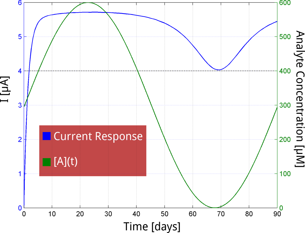
Fig. 1. A sinusoidally oscillating concentration of analyte (with period, T, of 90 days) in the feed stream (green) is plotted alongside the modeled sensor output (blue). For analyte changes on this timescale, current output traverses the entire range of the outputs from basal current of 4 $\mu$A to saturating current just under 6 $\mu$A— giving a fine-tuned output corresponding to analyte concentrations within the dynamic range.
However, for variations in analyte that occur on timescales of less than a month, the ‘memory’ of the system begins to interfere with our sensor’s ability to track fine changes in analyte concentration. As seen in Fig. 2 below, when oscillations in analyte concentration occur on the order of days, the response of our sensor approaches a constant output that accurately represents the time-average of the oscillating analyte concentration. Even though S.A.F.E. B.E.T. cannot track fine changes on these timescales, the ability to sense the time-averaged value represents a significant improvement over current detection methods that rely on ‘spot’ sampling—which often misrepresents the true analyte concentration.