"

From 2012.igem.org

• iGEM BsAs
  • The team
  • Official roster
  • Members
  • Where we come from

  • Safety
  • Key questions

  • Attributions
  • Attributions

  • Sponsors
  • Institutional

  Data Page
• Project
  • Synthetic ecology
  • Overview
  • Motivation
  • Design
  • Possible applications

  • Schemes
  • Crossfeeding
  • Independent Population Control
  • Cross-population control
  • Stochastic State Transitions

  • Modeling
  • Modeling synEcology
  • Advanced modeling

  Data Page
• Results and Devices
  • Strains characterization
  • Strains description
  • Fluorescence screening
  • Screening of strain proportion
  • Auxotrophy confirmation
  • Coculture in liquid medium
  • Revertant control
  • Trp basal production
  • Growth dependence

  • BBs design
  • Trp/His export devices
  • Backup devices
  • Preparing for sending

  • Testing
  • BioBricks testing
  • SynEco testing

  Data Page
• Human practices
  • Garage Lab
  • Spreading the word
  • Solving local problems

  • EMBO
  • Seeding SynBio in Latin America

  Data Page

Contents 1 Advanced modeling 1.1 Model Reduction: Quasy Steady State Approximation 1.2 Effect of the Hill coeffient 1.2.1 Relaxation time 1.2.2 Oscillations 1.3 Model Transformation: a new analysis 1.3.1 Stability of the regulation. 1.3.1.1 Oscillations Revised 1.4 Appendix 1.4.1 Model : SS solution 1.4.2 Transformed Model: SS

Advanced modeling

The standard procedure when studying the temporal evolution of a non-linear system is to try to determine all the possible types of trajectories in the phase space. First the nullclines and fixed points (FP) are found; then the latter are classified according to their stability; in the same way as a linear system. The goal is to qualitatively draw the trajectories for any initial conditions to see how the variables evolve. http://www.stevenstrogatz.com/books.html Nonlinear Dynamics And Chaos

Some relevant questions we can answer with this approach are:

• How is this behavior governed by the model's parameters?

• How do the trajectories change as the parameters vary? Does any new FP or close orbit appear?

There was a major difficulty in the analysis of the model because of the dimension of the problem - 4 variables. The analytical results yielded by the usual tools (nullclines, system linearization) could not be simplified so that all the relevant properties of the system could be understood in terms of the parameters.

We obtained the 4x4 Jacobian - evaluated in the FP - and later its eigenvalues. The expression found for them, a function of the relevant parameters, is too long and can't be simplified in a way that reveals changes in stability.

Besides that, we couldn't do a visual analysis of the nullclines to have a qualitative idea of what goes on.

1. A very common way to proceed in such a case is to reduce the model, ideally to a two-dimensional system. Sometimes one of the variables varies much more slowly/faster than the ones we are interested in, that it can be considered constant when studying the dynamics of the variables we are interested in. This is a standard procedure in the study of chemical reactions called Quasi Steady State Approximation.
2. We also noticed that the Hill coefficients are similar to one. So we explored the possibility of approximating them to one; is there a relevant change or not?

Model Reduction: Quasy Steady State Approximation

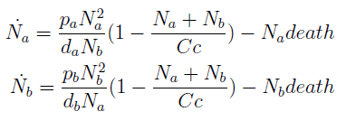
To gain some insight into the behavior of the model, we assumed that the variation of AA concentration in the medium is much faster than growth of the yeast populations.

(11)

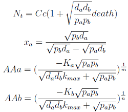
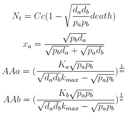
Therefore taking dAAj/dt=0, we re-wrote the Amino Acids as a function of (Na and Nb) in a reduced 2x2 model for the evolution of the populations.

(model_aprox)

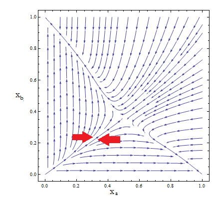
Thus a phase portrait for the nullclines and trajectories was drawn.

Figure 5. Phase portrait for the reduce model.

Although the reduced model presents the same fixed point, it’s a saddle point.

What does that mean? Pick any point for the plane; those are your initial conditions for the concentration of each population. Now to see how the community evolves with time follow the arrows - like a particle in a flow. No matter how close to the FP we start, the community is overtaken by one of the two strains.

• Only by taking i.c. along the stable manifold –direction marked between red arrows for clarification in Figure 5 – do we reach the FP we wanted as t → ∞.
• The stable FP are {Na → Nt, Nb → 0} and {Na → 0, Nb → Nt}.

This phase portrait is the one we'd expect for two species competing for the same resources. The Principle of Competitive Exclusion states that they can't typically coexist http://www.stevenstrogatz.com/books.html Nonlinear Dynamics And Chaos.

This is not a representation of auxotrophic community! Somehow we've landed on a Lotka-Volterra example.

The linearization of the set of ODEs around the FP yields instability regardless of the parameters. One of the eigenvalues is always positive.

{2death; death (1-√((pb pa)/(db da))/death)}

There is no agreement between the predictions found here and our simulations, that usually reach a non-trivial SS. We won’t pursue this reduction any further.

Effect of the Hill coeffient

How are the Kaa relevant when they haven't appear so far?

Originally we took both Hill coefficients equal to one in our numerical simulations, is close enough, right?

Well, the whole system didn't seem viable; it took over 100 hours for the fastest cultures to grow. Now using the fitted coefficients; the time scale becomes reasonable again.

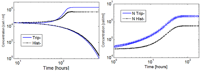
 Figure 6. Evolution in time of two cultures that only differ in the i.c.c. with both Hill coef = 1(left); and  both Hill coef > 1(right). 

• When n_ hill =1 only the culture with higher i.c.c. reaches a non-trivial SS. The other slowly dies.
• There is no clear difference between the cases with high and low i.c.c. for n_ hill =1.5. Note that they reach SS faster as well.

The survival of an auxotrophic community is dependent on both the apparent dissociation constants (Ks) and the Hill coefficient as shown clearly on Figure 6. There are two effects related to Hill parameters K and n_hill here:

Shorter time scale to SS.

Larger subspace of i.c.c. that lead to SS.

So when creating an auxotrophy, pick a nutrient with an appropriate Hill coefficient and K. Check the range of allowed i.c.c. estimating the values of the rest of the parameters. We could say that the model is more stable as more sets of initial conditions are susceptible of regulation.

Our case is similar to the one shown in figure 6 with both hill coefficients → 1. Region III is less sensitive to variations in the i.c.c. and therefore the actual Region III resembles the theorical one in Figure 4. When n_hill=1 is much smaller.

Relaxation time

Not only are we interested in predicting the fraction of each strain in the culture, we need this control within a time frame or the system is irrelevant.

Let’s call Τ the time it takes one of the populations to reach its SS value (relaxation time). We rely again on numerical simulations to obtain those set of parameters where Τ is less than 65 hours, for example.

Creating a mesh we explored the parameter space (p, ε) for different initial conditions i.c.c. to visualize when the model’s prediction and the numerical result of the simulations for the mole fraction in SS differ in an amount lower than the given error; before 65 hours. We won’t limit the mesh to Region III only.

We’ve taken 5% of the value as error; considering it an accurate estimation of an experimental measure’s precision.

For each set of conditions (p, ε,i.c.c.) we test the agreement between the proposed regulation and the NS.

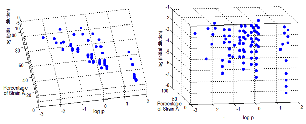
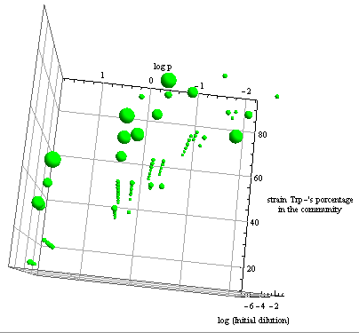
The first two graphs in Figure 7 are different orientations in space of a binary test, a blue dot indicates the points in this space where the error is smaller than 5%. Connecting the dots we see a pattern. This area in the parameter space where we can control the community through regulation has the same shape as Region III, although they don't overlap perfectly.

The green bubble's size in the third graph is a measure of the error in each point for the same NS; it ranges from 0.6 to 4%. The points with larger error are the ones in the area between Region II and III.

Some points well within Region III don't happen to comply with the established time limit. However there are enough points to see that all percentages are accessible with the model for the chosen precision. It's not necessary now, but a closer look at specific sections is possible with a higher point density matrix.

Figure 7. Scatter plot of the conditions under which the modeled auxotrophy leads to community control in under 65 hours with  a 5% precision.

Oscillations

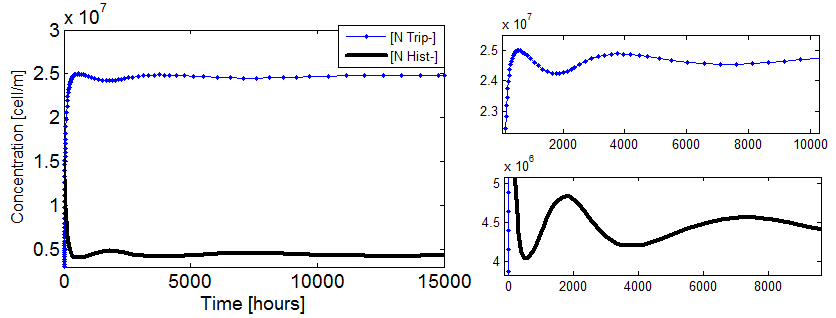
Damp oscillations are observed!!

This interesting effect was found while doing random searchs through our paramater space. It appears if:

• the initial concentration of AA in the medium are of the order of the Kaa and
• the parameters that regulate the production and export of AA are from region II in Figure 4 and
• we work with the approximate model where both n_hill= 1.

 Figure 8. Evolution of the two populations in the community vs time when the conditions above are met. Both populations fluctuate with time in
 such a way that Nt remains constant. 

We were unable to numerically find parameters where the oscillation period was shorter.

Model Transformation: a new analysis

Let’s review what we’ve learned so far from our system.

• Seems stable,

• capable of oscillations,

• there are two cases with a stable population and a defined mole fraction for each strain, one where the AAs are in SS and one where they aren’t.

• The set of i.c. for which the culture thrives is dependent on the Kaa and Kbb.

Yet all this information is not so trivial to find – especially the oscillations discovery was a fluke.

There had to be a transformation where all these properties were more accessible or evident.

What we did so far was to write the results in more convenient variables.

Now we will try to find a transformation to a new set of variables, whose evolution is simpler to study and write a new set of ODEs for them.

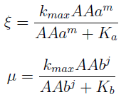
For instance the AAs only appear as the argument of Hill functions, so why not just work with those rations. We defined:

(12)

This is better because now ξ is constant when:

1. AAa reachs steady state.

1. Na exports more that could Nb possibly adsorb and AAa accumulates in the medium. For AAa >> Kaa the ratio ξ → k_max.

The same argument is valid for μ.

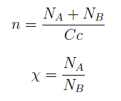
Then we take the obvious choices to describe the percentage of each and the total population of the community.

(13)

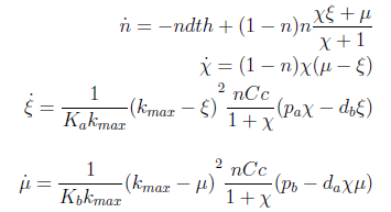
Now we must find differential equations that describe their dynamic.

For example: (14)

and

(15)

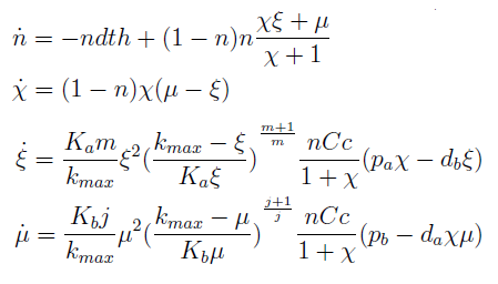
The new set of ODEs with m,j >1 is:

(transf_model)

The AAs can be zero, so can the new variables. Rewriting the equation we see that each ratio is elevated to 2- (s+1)/s > 0 for s > 1; so the variables are not really in the denominator.

The model with m=j=1 is in the Appendix.

Admittedly, this new set of differential equations looks like more trouble; however many of the properties we struggled with before are evident in the new version of the model.

• χ stop growing (is constant) if and only if μ = ξ, since n=1 doesn’t satisfy the DE for n.

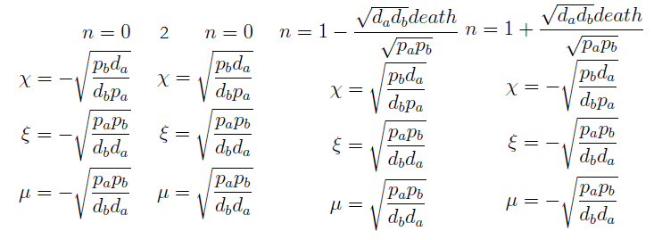
• This system has 4 solutions. Only have two biological significance, the ones we already know: Nt → 0 and equation (3) in the old variables.

• If ξ = k_max, the culture again reaches a SS, but the fraction χ is indeterminate.

Here’s the great improvement over the old variables. The SS for χ, ξ and μ is independent of n; moreover the conditions for which their DE equal zero follow directly from a visual inspection of the ODEs. The nullclines are independent as well and just as easy to determine and plot. Now we have a reduction in the system's dimension. Same SS as before but in a 3x3 system can be analyzed visually,

• We can represent the vector field in space and track a trajectory that starts at (χ0, ξ0, μ0).
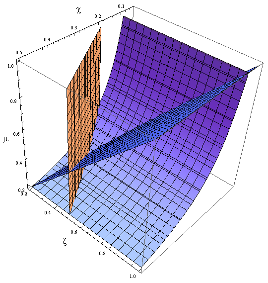
• We can plot the nullclines, see where they meet- Figure 9; do a quick stability test by checking the sign of the vector field around the FP.

Figure 9. Nullclines for the reduced model in the new variables χ, ξ and μ.

Stability of the regulation.

Let’s directly go to the linearization of our 3 ODEs close to the FP where there is regulation through the auxotrophy.

We said that n wasn’t relevant to the fixed point's location, but now we have to consider it while examining the eigenvalues.

Once again the expresion for the three eigenvalues γ is very long. We replace the mayority of the parameters with the value we estimated, and n for its SS value - though this is not always correct.

We are able now to study the stability of the FP when we vary pa and pb.

Reminder: The FP is not a stable node if at least one of the eigenvalues is positive.

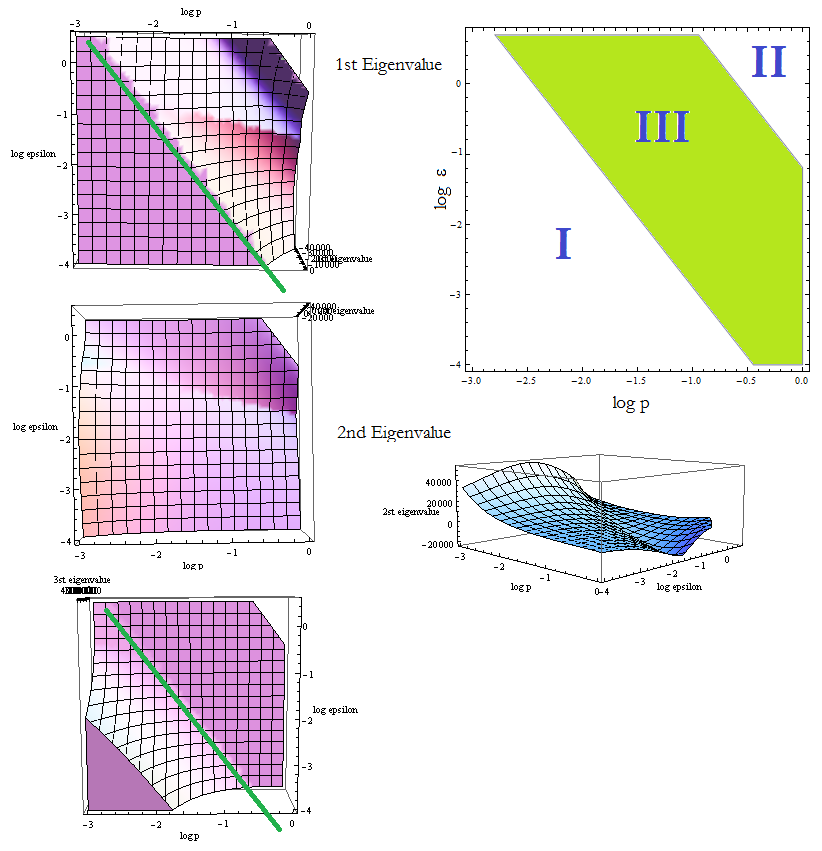
Figure 10. Visual aid to determine how the eigenvalue's sign changes with model's parameters p and ε. 
The division of the parameter space previously found is also plotted to facilitate comparisons.

Figure 10 shows a top view of the eigenvalues vs (p,ε). All the information we need can be read from them. The first and third γ present a clear change in behavior that we accentuated with the green line, we present also a side view for the second γ since it's not so obvious. The eigenvalues change sign there; positive below and negative above the line.

• The region where the eigenvalues are positive, corresponds to a unstable FP. Comparing Figure 10 with Figure 4 reveals that we are in fact in what we called Region I. The trajectories tend to another FP: Nt → 0.

• The three eigenvalues are negative above this line we drew: the FP it's a stable node in this region of the parameter space. This corresponds with Region III.

• There's another area up in the right corner where the values are not plotted. Taking (p, ε) from that region we obtain complex eigenvalues; this is well within Region II. There's a dark region for the first eigenvalue before it becomes complex; it's likely the values from II that do have real negative eigenvalues.

Next are some examples of complex γ:

• (1,1) → {-35537.4 + 85795. i, -9334.41 + 5389.23 i, -0.0119048 - 3.99219*10^-9 i}
• (0.74,0.74 ) → {-2142.41 + 5172.24 i, -513.323 + 296.37 i, -0.0119049 - 7.1472*10^-8 i}

In these cases the solutions for (n (t), χ(t), ξ(t), μ(t))are not real numbers. These coincide with the values that made MATLAB scream during the NS: there is no real solution.

Oscillations Revised

The oscillations in Figure 8 correspond to the model where the Hill coefficients are set to 1. Though we tried, we couldn't manually find a set of parameters and i.c. so that they appear when using the model with the correct Hill coefficients.

Is this always the case? Could we find the answer using the new variables?

We found a tendency by sampling random values (p,ε) from the region where the eigenvalues are complex and i.c. (χ0, ξ0, μ0). So far the examples from the section above are representative of our findings.

It seems that when when n_hill > 1, the complex eigenvalues of the linearization around the FP lead to complex solutions for the temporal evolution of the variables because they are not complex conjugates.

Still, this doesn't exclude the possibility of bifurcations that change the stability or simply later finding a small subset where oscillations occur. Just that we were unable to completely characerize the behavior due to the complexity of the problem.

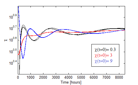
The next figure shows some of the i.c. for which damp oscillations exist in the first case.

Figure 11. Oscillations in the fraction of each population when the AAs are initially saturated.

The oscillations obtained for different initial conditions: χ0 = 0.3, 3, 9 in black,red and blue are presented in Figure 11. We varied the initial total population through n0= 1:2,1:20,1:200 for each χ0 and found little variance in such case.

The eigenvalues obtain have for the parameters in Figure 8 and 11 are:

(0.5, 0.5) → {-0.0734764, -0.0206177 - 0.0211589 i, -0.0206177 + 0.0211589 i}

The second and third are complex conjugates with real part < 0. Together they generate what is called a stable spiral in the eigenvector space: all close trajectories are attracted to it; the flow is the like water whirling in a sink.

This means that when we plot χ vs time we see that the oscillations around a value grow smaller. χ tends to that value as t → ∞.

The more distintive characteristics of these damp oscillations are:

1. AA must be initally saturated.
2. The period is huge: over a thousand hours; well above the 50 hour given by the linearization.
3. The period is not constant, this is due to the non-linear nature of the system.
4. There is a dependance with the initial fraction χ0 but not on the intial dilution n0.

Appendix

Model : SS solution

1. Nt -> 0

2.

3.

Transformed Model: SS

Steady states

The model obtained when m=j=1 differs:

However the solutions remain the same.