Team:TU Darmstadt/Modeling MD
From 2012.igem.org
(→3KVN in lipid layer) |
(→References) |
||
| Line 122: | Line 122: | ||
==References== | ==References== | ||
| - | *Molecular mechanical and molecular dynamical simulations of | + | *Molecular mechanical and molecular dynamical simulations of glycoproteins and oligosaccharides. 1. GLYCAM 93 parameter development |
| - | glycoproteins and oligosaccharides. 1. GLYCAM 93 parameter development | + | |
Woods RJ, Dwek RA, Edge CJ, Fraser-Reid B (1995) J.Phys.Chem. | Woods RJ, Dwek RA, Edge CJ, Fraser-Reid B (1995) J.Phys.Chem. | ||
99, 3832-3846 | 99, 3832-3846 | ||
Revision as of 11:44, 26 September 2012
| Homology Modeling | | Gaussian Networks | | Molecular Dynamics | | Information Theory | | Docking Simulation |
|---|
Contents |
Molecular Dynamics
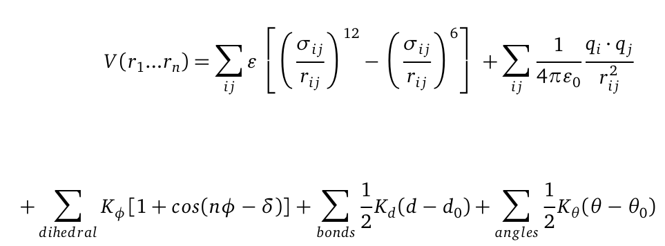
Molecular dynamics (MD) is one of the most common tools in computational biology. MD simulations solve the classical newton’s equations of motion. For the computation we need to calculate all forces acting in our system. The Forces during simulation are calculated from a force field, that contains information about the potential energy of the involved molecules. For illustration the potential is computed as follows:
The first term represents a a Lennard-Jones (LJ) potential. It approximates the interaction between a pair of neutral atoms or molecules. The second term is a coulomb potential between a pair of atoms i and j. The last terms describe bonds and angles potentials. Due to experimental data and quantum chemical calculations the force-field parameters can be identified.The quality of MD simulations is largely depending on the applied force field. In physics, a force field is a vector field which describes range dependent all non-contact forces acting on a particle. In biochemistry a force field is a collection of mathematical functions and parameters which describe the potential energy of particles (atoms and molecules) in a defined system. For our simulations we used the AMBER (Assisted Model Building with Energy Refinement) force field which was especially developed to describe proteins and DNA.
Goal
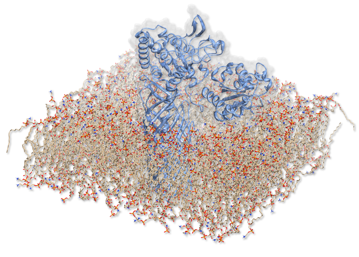
In order to characterize the enzyme construct and to simulate its complex behavior, MD was required to study the interactions. Hence to the degradation of PET, our Team designed a sophisticated protein-construct. This construct is a fusion protein containing a degradation module (PDB :1CEX, pnB) and EstA (PDB id: 3KVN), a membrane bounded beta-beryl. Moreover, this construct is exposed at the outer membrane of our bacteria. Hence, we quantified the dynamic nature of our degradation protein with coarse-grained methods. We have to quantify the motion within this construct surrounded by its native environment. We first have to recreate the situation that puts the fusion protein into a membran layer. This results in a complex simulation setup, which was nonetheless performed to access crucial information about the enzyme.
Methods
We used Yasara Structure simulation protocol for membrane protein. But we changed parameters and settings to fit our fusion protein-construct.
We have to define our system and set some simplifying constrains: First we define the system as isolated from the surrounding, so to keep the number of a particles (atoms) constant; The simulated volume clearly defined, but periodic. This causes a particle that would leave the volume on one side, to re-enter it again on the opposite side.
Protocol for the simulation of 1CEX fused with 3KVN in lipid layer
Setting the Parameters
- Forcefield: AMBER03
- Periodic simulation box
- Membrane composition: 100 % phosphatidyl-ethanolamine (PEA)
- Equilibration period = 250 ps
- duration= 3.5 ns
- temperature= 298K
- Membrane height = 43 nm
- Height of the hydrophobic membrane core = 28 nm
- Periodic simulation box
- duration : 5 ns
Flow
- Scanning the protein for hydrophobic aa
- Calculate the size of the membrane
- Make a short MD Simulation of the membrane
- Insert the protein into the membrane
- Adding water to the Scene
- Performing pH neutralization experiment
- Energy Minimisation
- Keep the Protein rigid
- Equilibration of the solvent
- Equilibration of the membrane
- Protein free and simulating
Now we are ready to start the simulation. For each of the molecules in our simulation box we solve the equation from above and find out the forces which act on them. Then the forces are applied on the molecules for a short time period (femto seconds; fs) which results in a movement. A snapshot is taken of each atom position and the whole calculation starts over again. This calculation is repeated for a great number of time steps amd the result is a motion study of all atoms in the simulation box, an MD simulation.
Analytics
RMSF
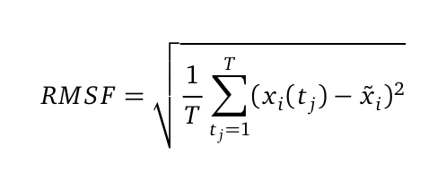
The Root mean square fluctuation (short: RMSF) can be computed as followed:
where T is the duration of the simulation (time steps) and x i (t j) the coordinates of atom x i at time t j. Now we are calculating the sum of the squared difference of the mean coordinate x i and x i (t j). Next we divide the sum to T and extract the root of it. Hence we are able to calculate the fluctuation of an atom with its mean in trajectory files. The RMSF was computed from the atomic coordinates of the Cα in R using the bio3d library.
RMSD
The Root mean square deviation (short: RMSD) can be computed as followed:
where n is the number of atoms (Cα or backbone atoms). V i is defined as the coordinates of protein V atom i. Here, the RMSD is used to quantify a comparison between the structures of two protein (v and w) folds. The RMSD was computed from the atomic coordinates of the Cα in R using the bio3d package.
Results
1CEX fused with 3KVN in lipid layer
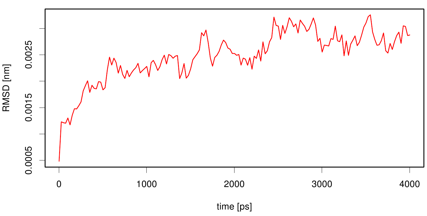
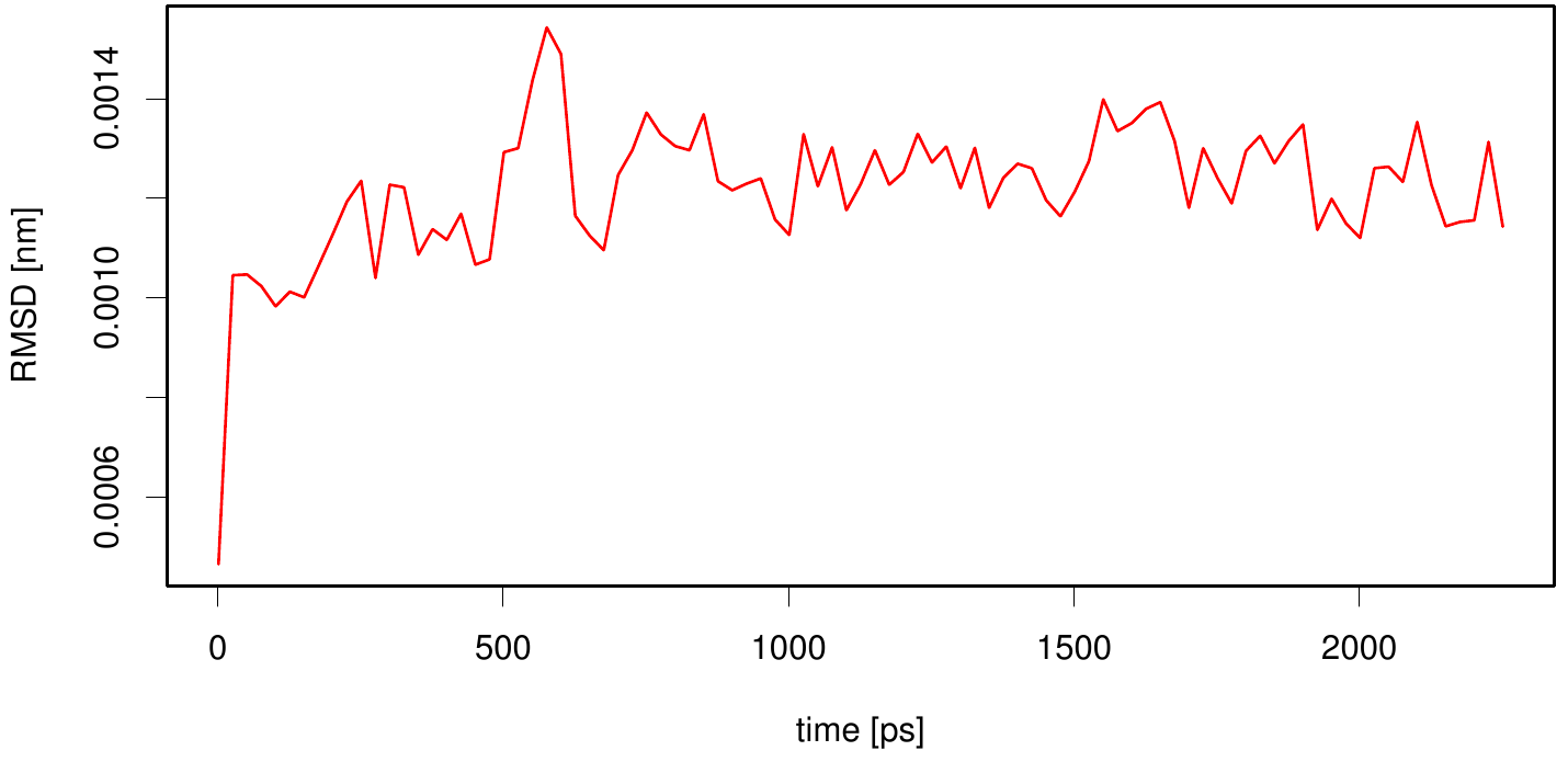
Here we calculate the RMSD as a function of time. We use the starting structure as reference and after a least square fit we compute the RMSD of every frame in our trajectory. We observe that the RMSD value converges after a period of time. This indicates that our simulation is stable.
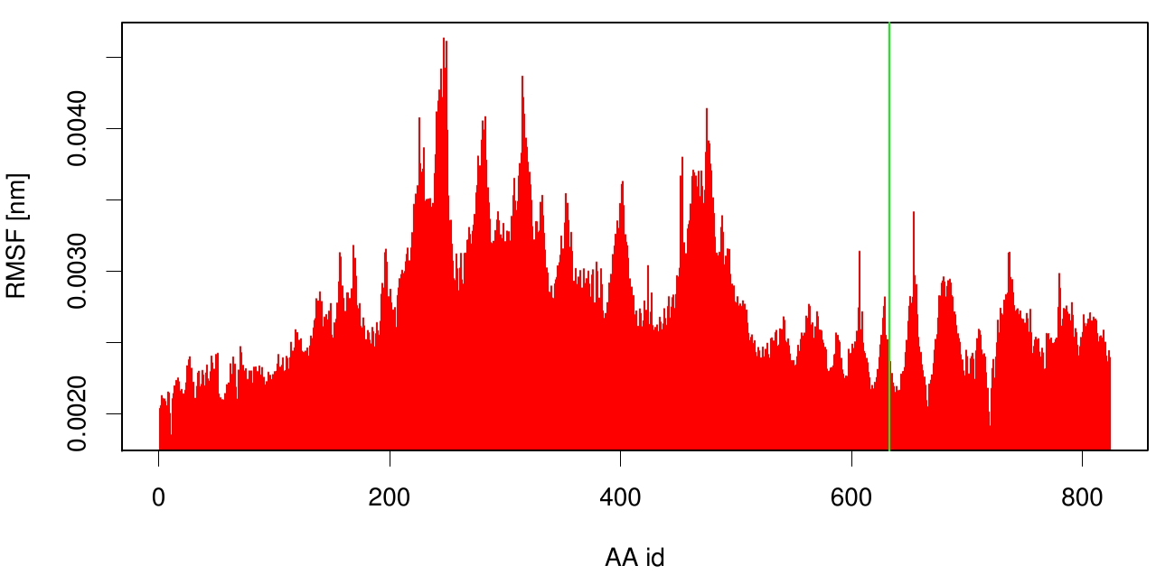
Here the RMSF is shown as a bar plot of residue numbers. The green bar reveals the fusion site of 3KCV and 1CEX. Interestingly, we can observe that the membrane part (3KVN) exhibits a higher fluctuation than our degrading enzyme (1CEX).
- For illustration you can watch a movie clip from the MD Simulation hosted on our server:
http://bioserver.bio.tu-darmstadt.de/igem_data/1CEX_3KVN_Chimere.mpg
3KVN in lipid layer
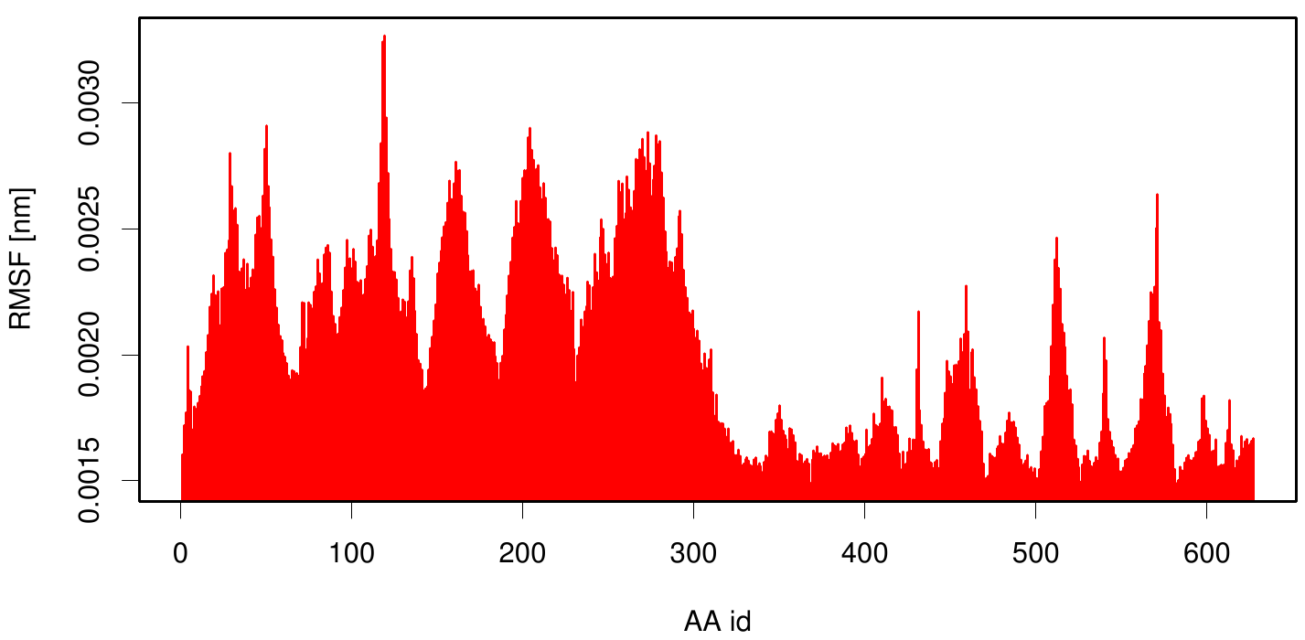
Interestingly, if we compare the outer membrane region (C-terminal) of 1KVN with the membran bounded simulation we observe smaller RMSF values.
References
- Molecular mechanical and molecular dynamical simulations of glycoproteins and oligosaccharides. 1. GLYCAM 93 parameter development
Woods RJ, Dwek RA, Edge CJ, Fraser-Reid B (1995) J.Phys.Chem. 99, 3832-3846
- Krieger, E., Darden, T., Nabuurs, S. B., Finkelstein, A., & Vriend, G. (2004). Making optimal use of empirical energy functions: force-field parameterization in crystal space. Proteins, 57(4), 678-683. Wiley Subscription Services, Inc., A Wiley Company. Retrieved from [http://www.ncbi.nlm.nih.gov/pubmed/15390263 link]
- Multiscale Simulation Methods in Molecular Sciences,Lecture Notes,edited by Johannes Grotendorst, Norbert Attig, Stefan Blügel, Dominik Marx,ISBN 978-3-9810843-8-2
 "
"
