Team:Buenos Aires/Project/Model
From 2012.igem.org
(→Model Analysis) |
(→Die or thrive?) |
||
| Line 208: | Line 208: | ||
[[File:bsas2012-modeling-eq7.png]] | [[File:bsas2012-modeling-eq7.png]] | ||
| + | |||
| + | [[File:bsas2012-modeling-fig3.5.png]] | ||
Figure 3. | Figure 3. | ||
| Line 243: | Line 245: | ||
Our case is shown in figure 3 with both hill coefficients are > 1 and we haven’t found the same variability in the behavior. It’s insensitive to change in the same range! And it’s faster! | Our case is shown in figure 3 with both hill coefficients are > 1 and we haven’t found the same variability in the behavior. It’s insensitive to change in the same range! And it’s faster! | ||
| - | |||
=== Relaxation time=== | === Relaxation time=== | ||
Revision as of 22:49, 23 September 2012

Contents |
Modeling a synthetic ecology
To gain insight into the behavior of our crossfeeding design, to understand which parameters of the system are important, and to study the feasibility of the project, we decided to implement a model of the system. We found this interesting per se, as the model we need is that of a microbial community, an ecology.
The mathematical modeling of ecological system is an active field of research with a very rich and interesting history; from the works of Lotka and Volterra, who modeled predator-prey dynamics with ordinary differential equations, to Robert May’s chaotic logistic maps. In fact a lot of synthetic systems of interacting bacteria created in recent years were used to study these sort of models.
The crossfeeding model
In the crossfeeding design, each strain produces and releases to the medium an aminoacid the other strain(s) need to grow. The growth rate of each strain depends on the aminoacid (AA) concentration of those AA it can’t produce. In turn these concentrations depend on the abundance of the other strains. Therefore the growth of the strains is interdependent.
For simplicity and to be consistent with the experimental work, we decided to model two interacting strains, one that produces tryptophan (Trp) but requires histidine (His), and another that produces His but requires Trp.
We decided to use ordinary differential equations to model the system. This is a normal approach when studying population dynamics of this kind.
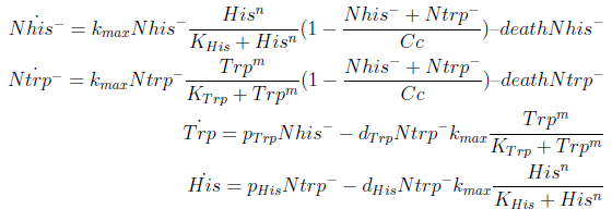
The model has four variables: [Nhis-] : the concentration of histidine dependent (Trp producing) yeast cells, in cells per ml [Ntrp-] : the total amount of tryptophan dependent (His producing) yeast cells, in cell per ml [his]: the concentration of histidine in the medium, in molecules per ml [trp]: the concentration of tryptophan in the medium, in molecules per ml.
To build the model we did the following assumptions:
- The growth rate of each strain depends on the concentration in the medium of the AA they can’t produce. As the concentration of this AA in the medium increases, so does the growth rate of the strain, until it settles at the growth rate observed in optimal conditions (doubling time of 90 min for yeast).
- There is a maximal density of cells the medium can support
- Each cell has a fixed probability of dying per time unit
- Each cell releases to the medium the AA it produces at a fixed rate
- Each strain only consumes the AA it doesn't produce
- The system reaches steady state.
Subsubsection
In the equation for the temporal evolution of each population we take the growth rate as a Hill function of the amount of AA to which the population is auxotrophic. The function represents the stabilization of the rate to a 90 minutes cell division cycle (kmax).
K_AA is the apparent dissociation constant.
The second term accounts for other factors, not explicit in our model that can limit the concentration of cells in a given volume (capacity) enabling the population to reach equilibrium. Given that our model relies on nutrient deficiency we can't rule out starvation so we added a term related to cell death.
The terms in the equations for the evolution of each [AA] in the medium are the fluxes of AA entering and leaving the medium. Each rate p is a measure of the AA produced and exported in the form of a protein by a cell. In our simulations it is defined as a fraction of the calculated maximum of elongation events.
The second term is the flux leaving the medium and entering the auxotrophic cells. We have assumed that the total amount of AA absorbed, d, during the cell cycle time τ is the required to build the daughter. One of the hypotheses built into our model is that τ will vary greatly with the concentration of nutrients available. We've used
The amount of AA entering the cells that produce it was considered negligible.
Steady State Solution
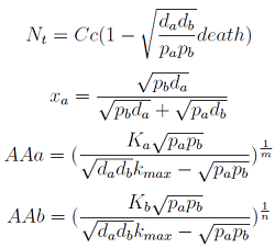
The 4 equations in [] were equaled to zero and the non-linear algebraic system solved using MATEMATICA to find their equilibrium values.
Here we change the notation a little to two generic strains a and b where population Na produces amino acid a, etc. We are interested in the value of the cell populations in equilibrium, more importantly in the fraction of each population. Thus a change was made to more convenient variables: the sum of both population and a strain's molar fraction.
{N_{a} ; N_{b}} → { N_{t} , x_{a} }
Only 3 fixed points were found for the system {Nt, Xa, AAa, AAb} (See Appendix) That means that for some solutions it’s not true that the four variables reach a steady state or equilibrium. There are initial conditions for which some of the variables will not stop growing!
- The first solution is clear. The culture will not thrive under certain conditions… to be determined!
- The second one has no physical relevance since it yields negative concentrations for the Amino Acids.
- The third one is the significant one. However the concentrations of Nt and AA can be negative; we must work within the region where is positive.
Regulation
Note that the percentage of each population in the community is a function of √((da pa)/(db pb)).
In particular
For positive values of d and p the range of the function is (0; 1), so far it’s consistent with what we expect.
The percentages of the strains in the culture in equilibrium are regulated by the production and export of AA – represented in the model through pa and pb; independent of initial conditions!!
In fact we need only know the ratio between these two parameters to control it:

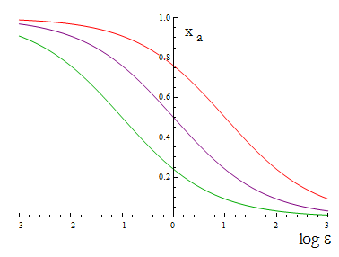
The next figure illustrates how the mole fraction x_a varies with the variable ε.
Figure 1. Mole fraction x_a as a fucntion of the ratio of protein export for values of D=0.1,1,10.
The ratio D is fixed for two A.A., this determines the range of percentages of each strain accessible for any selection of biobricks.
Parameters
The parameter estimation process is shown in xx section(linked)
| Value | Units | |
| kmax | 0.4261 | 1/hr |
| K his | 2.588e16 | AA/ml |
| K trp | 1.041e16 | AA/ml |
| n his | 1.243 | |
| n trp | 1.636 | |
| Cc | 3.0 10^7 | cell/ml |
| death | 3 to 7 | days |
| p his | p 2.16e8 | AA/ cell hr |
| p trp | p ε 2.16e8 | AA/ cell hr |
| d his | 6.348e8 | AA/cell |
| d trp | 2.630e7 | AA/cell |
Table 1.
Model Analysis
The standard procedure when dealing with a non-linear system is to find the fixed points(FP) and later analyze their stability; same as with a linear system. The goal is to determine all possible trajectories, i.e. for any initial conditions how do the variables evolve? How is this behavior governed by the model’s parameters?
How do the trajectories change as the parameters vary?
Does any new FP or close orbit appear?
There was a major difficulty in the analysis of the model because of the dimension of the problem - 4 variables. The analytical results yielded by the usual tools (nullclines, linearization) could not be simplified so that all the relevant properties of the system could be understood in terms of the parameters.
We obtained the 4x4 Jacobian - evaluated in the FP - and later its eigenvalues. The expression found for them, a function of the relevant parameters, is too long and can’t be simplified in a way that reveals changes in stability, etc.
Besides that, we can’t do a visual analysis of the nullclines to have a qualitative idea of what goes on.
A very common way to proceed in such a case is to reduce the model, ideally to a two-dimensional system. Sometimes one of the variables varies so slowly or so much faster than the ones we are interested in, that it can be considered constant when studying the dynamics of the rest.
This is a standard procedure in the study of chemical reactions called Quasi Steady State Approximation.
- QSSA: the variation of AA in the medium is much faster than the yeast‘s populations. Initially
Therefore taking dAAj/dt=0 we can rewrite the AminoAcids as a function of (Na,Nb) in a reduced 2x2 model for the evolution of the populations.
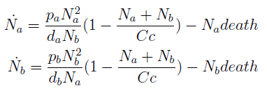 Thus a phase portrait for the nullclines and trajectories was drawn.
Figure 2
Numerically we see that while [] is true, the four variables reach SS at the same time. Indeed, although the reduced model presents the same fixed point, it’s unstable. We see in Figure that for any i.c. the community is overtaken by one of the two strains. This is not a representation of auxotrophic community!
Another trick we tried was to replace the AAs with their SS value as oppose to a function like was done above. There is still no agreement between the predictions found and the simulations.
We can’t seem to escape to a more elegant and simple system.
- We’ve also noticed that the Hill coeficients are similar to one. We explored the possibility of approximating them to one; is it a relevant or not?
Simulations
We’ve relied on numerical simulations to explore possible behaviors.
To run the simulations all that is left is to choose values {p, ε, i.c.}.
Since this is merely a framewok we have taken values p from a log scale from -3 to 1.
ε was ranged from 0.0001 to 4; which varies the fraction of each population from 10% to 90%.
Cells’ initial concentration: dilutions from 1/10000 to 1/100 of the capacity (Cc).
AAs’ initial concentration: null.
Die or thrive?
Some basic properties were observed by simplifying the system; we wanted to check that our model was sound.
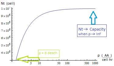
Nt=Cc (1-(d death)/p)
Figure 3.
The condition for culture growth is λ > 1. This ratio λ between two rates determines whether the system is able to produce and absorbed the nutrients needed for the cell cycle before its death. If it doesn’t hold the culture dies, ie the total amount of cells is negative.
The other condition is related to extracellular AAs. Let’s define
The concentration of extracellular AAs is positive only if δ < 1. In fact as δ -> 1 the concentration -> infinity because δ = 1 is a vertical asymptote. This ratio δ between two rates is related to our proposed regulation; if the amount of nutrients produced exceeds the required one for a 90 minutes cycle, the medium is saturated. Then the regulation fails.
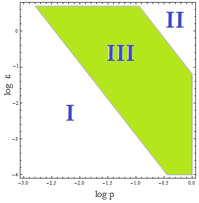
Uniting the conditions we find that p and ε are bound by:
Figure 4. Regions in the parameter space that present different types of solutions defined by the conditions in X.
- Region I
- Region II
- Region III
Yet the picture is not whole. We’ve noticed that the culture’s survival in region III is also dependent on the Ks even though is not explicit in the formula above. This is reasonable considering that it introduces another time scale. Not only have the cells to produce and absorb the required amounts of AA before they die, but their growth is restricted by the concentration of AA in the medium. The cells must produce amino acids not in the order of what they will absorbe (d) but the required one to jump start their growth (K) in the time frame to insure their prosperity.
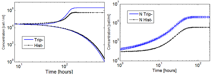
Figure 5. Evolution in time of two cultures that only differ in the value of the Ks for n_ hill =1 (left)and n_hill >1 (right).
When n_ hill =1 only the one with lower Ks reaches a non-trivial steady state (SS). The other slowly dies. However for n_ hill =1.5 there is no difference between the cases with high and low Ks. Note that it reaches the SS faster as well.
The survival of an auxotrophic community is dependent on the apparent dissociation constants(K) and the Hill coefficients as shown clearly on Figure 5.
So when creating an auxotrophy, pick a nutrient with an appropriate Hill coefficient and K. Check the range and stability of your model estimating the values of the rest of the parameters.
Our case is shown in figure 3 with both hill coefficients are > 1 and we haven’t found the same variability in the behavior. It’s insensitive to change in the same range! And it’s faster!
Relaxation time
Not only are we interested in predicting the fraction of each strain in the culture, we want it within a time frame. Let’s call Τ the time it takes one of the populations to reach 90% of its SS value.
This is easier to find given an expression Ni(t). However, we rely on numerical simulations.
Creating a mesh we explored the parameter space (p, ε) for different initial conditions to visualize when the model’s prediction and the numerical result of the simulations differ in an amount lower than the given error; before 65 hours.
We’ve taken 5% of the value as error; considering it an accurate estimation of an experimental measure’s precision.
Figure 6.
Oscillations
One interesting effect appears if the initial concentration of AA in the medium is of the order of the Ks. Damp oscillations were observed!!
Figure 7.
The next figure present the oscillations for different initial dilutions. We found that the more diluded the initial culture, the more damped the oscillations.
Figure 8.
Parameter selection
We've estimatated values for all the parameter in the model to check is viability.
- The Ks found in the equations are a measure of the concentration of A.A. in the medium required to reach half the maximum rate of growth. Curves OD vs [AA] were measured experimentally for each amino acid and the data fitted to a Hill equation using MATLAB’s TOOLBOX: Curve Fitting Tool.
Figure aux his and aux trp.
The values were taken from the fits are
His- :
      K_dil =     0.3279
      ODmax =      62.53
      n =          1.243
 R-square: 0.9376
Trp- :
      K_dil =     0.1770
      ODmax =      57.46
      n =          1.636
 R-square: 0.9905
The results were then converted to the units chosen for the simulations.
K = K_dil * [AA 1x] # Avog / (Molar mass AA), where [AA 1x] = 0.02 mg/ml
- K trp= 0.1770 * 5.88e16 AA / ml.
- K his= 0.3279 * 7.8e16 AA / ml.
- The capacity of the system taken in the model is the one often used in the lab that works with these yeast strains:
- Cc= 3e7 #cell/ml.
- The death rate was taken between 3 and 7 days.
- The rate of “production and export” was given a top value (P_MAX) 1% of the maximum estimated number of elongation events for a yeast cell per hour. Our model does not explicitly include time as a variable, that means that the production is switched ON all the time.
Elongation events (peptidil transferase reactions): 6e6 1 / cell sec [ref]
P_MAX = 2.16e8 1/ cell hour
These parameters will be regulated experimentally (ε , p) to alter the fraction between populations.
- p trp = p* ε*2.16e8 aa / cell hour
- p his = p*2.16e8 aa / cell hour
where p < 1 controls the fraction of the top value and ε the ratio between the export of each amino acid.
- d is the total number of amino acids in a yeast cell –same as the ones needed to create a daughter -per cell:
d = # A.A. per cell = (mass of protein per yeast cell [ref]) * relative abundance of AA * # Avog / AA's molar mass.
- d trp= 2.630e7 AA / cell
- d his= 6.348e8 AA / cell
Appendix
solutions model1
Sol2
Sol3
 "
"
