Team:UC Chile/Cyanolux/Modelling
From 2012.igem.org
(Difference between revisions)
| (25 intermediate revisions not shown) | |||
| Line 1: | Line 1: | ||
{{UC_Chile4}} | {{UC_Chile4}} | ||
| + | <h1>Why Modelling?:</h1> | ||
| + | Synechocystis transcriptional circadian oscillation makes it an exceptional chassis if time control of synthetic metabolic processes is desired. | ||
| + | Nevertheless, the functionality of some of these processes depends upon precise timing. | ||
| + | While there are hundreds of genes known to oscillate in Synechocystis genome -each with its own peak, strenght and amplitude- it can be tricky to choose the right ones. | ||
| + | Here is where our modeling approach comes on stage. | ||
| - | < | + | <h1>Model Overview:</h1> |
| - | + | <h2>Model Application</h2> | |
| + | Our model works as a user-friendly black box. The user´s input is the desired time of protein concentration peak and the program´s output is a list of suggested promoters. | ||
| + | It can be adjusted to take as input the time on which enzymatic products concentration peaks , or to maximize an intermediate metabolite that depends not just on production but also consumption. | ||
| + | Finally, its logical design can be applied to any other organism that exhibits circadian oscillation. | ||
| + | <html><center><img src="https://static.igem.org/mediawiki/2012/9/93/Boxextended.jpg" align="left" width="720"></center></html> | ||
| - | |||
| - | |||
| - | |||
| - | |||
| - | |||
| - | |||
| - | |||
| - | + | <h2>What´s inside the box?</h2> | |
| + | <html><center><img src="https://static.igem.org/mediawiki/2012/c/c0/Openbb.jpg" align="left" width="320"></center></html>We took all the microarray data available of promoter of Synechocystis grown on normal conditions. Conveniently, these arrays already have a filter: they only contain cycling promoters | ||
| + | |||
| + | |||
| + | |||
| + | |||
| + | |||
| + | |||
| + | |||
| + | |||
| + | |||
| + | |||
| + | |||
| + | |||
| + | |||
| + | |||
| + | |||
| + | |||
| + | |||
| + | |||
| + | |||
| + | |||
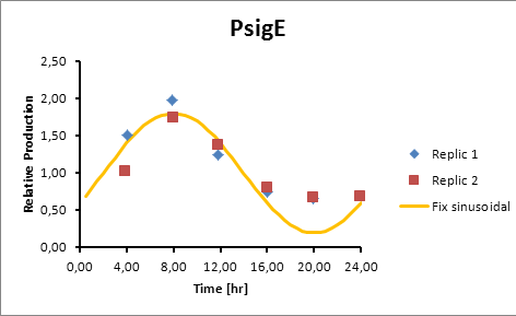
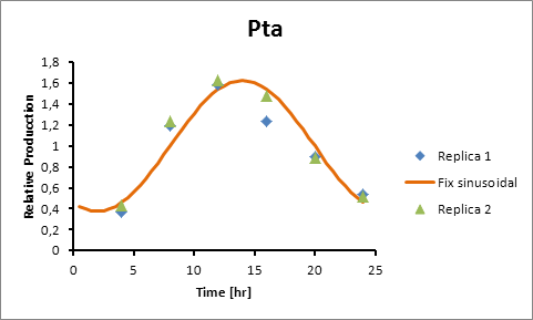
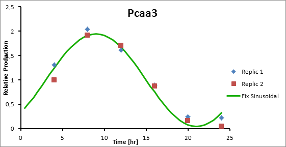
| + | The microarray data points were adjusted by a least squares algorithm into sine functions for each promoter. | ||
| + | <html><center><img src="https://static.igem.org/mediawiki/2012/2/2f/Equa1.scheme.jpg" align="left" width="606"></center></html> | ||
| + | <br /> | ||
| + | <br /> | ||
| + | Where k, theta and y are parameters to adjust. | ||
| + | x is protein concentration | ||
| + | <br /> | ||
| + | <br /> | ||
| + | <br /> | ||
| + | <br /> | ||
| + | <br /> | ||
| + | |||
| + | This equation accounts for protein production and its included into this form of universal balance equation: | ||
| + | <html><center><img src="https://static.igem.org/mediawiki/2012/2/24/Equa2.2.jpg" align="left" width="706"></center></html> | ||
| + | <br /> | ||
| + | <br /> | ||
| + | <br /> | ||
| + | <br /> | ||
| + | <br /> | ||
| + | <br /> | ||
| + | <br /> | ||
| + | <br /> | ||
| + | Where HL is protein´s half life | ||
| + | <br /> | ||
| + | |||
| + | The resulting plot of this equation predicts protein concentration over time. | ||
| + | |||
| + | As a complement, we developed a list of relative promoter strengths. We took one promoter present in all datasets to make a relative scale, then, we transformed it to an absolute scale using a promoter quantitatively characterized in literature by comparing it to the relative scale promoter. | ||
| + | |||
| + | <h1>Extended Model</h1> | ||
| + | The approach can be extended to consider as input the product of the protein enzymatic activity instead of the protein itself. | ||
| + | |||
| + | Moreover, it can be adjusted to a two-protein model in which protein 1 produces the metabolite and protein 2 consumes it. | ||
| + | |||
| + | <h1>Applying the model: Synechocystis promoters</h1> | ||
| + | We applied our model to solve the question of which promoters should we use to meet our [https://2012.igem.org/Team:UC_Chile/Cyanolux/Project_short#Strategy strategy goals] | ||
| + | |||
| + | The results are shown below: | ||
| - | |||
Promoter Peak hour | Promoter Peak hour | ||
| Line 33: | Line 93: | ||
sigE production=0,8028*sen(π(t-2)/12)+1 | sigE production=0,8028*sen(π(t-2)/12)+1 | ||
| - | [[File:sigeprodction.jpg]] | + | [[File:sigeprodction.jpg|center]] |
Pta production=0,6246*sen(π(t-8)/12)+1 | Pta production=0,6246*sen(π(t-8)/12)+1 | ||
| - | [[File:ptaproductoihj.jpg]] | + | [[File:ptaproductoihj.jpg|center]] |
Pcaa3 production=0,9493*sen(π(t-3)/12)+1 | Pcaa3 production=0,9493*sen(π(t-3)/12)+1 | ||
| - | [[File:pcaa3production.jpg]] | + | [[File:pcaa3production.jpg|center]] |
<font size="3">Solving ODE’s</font> | <font size="3">Solving ODE’s</font> | ||
| Line 56: | Line 116: | ||
As there is no entries nor exits (closed system) the expression becomes | As there is no entries nor exits (closed system) the expression becomes | ||
| - | + | Generation-consumption= accumulation | |
For LuxAB we know | For LuxAB we know | ||
| Line 71: | Line 131: | ||
Using Matlab to solve this ODE | Using Matlab to solve this ODE | ||
| - | + | ||
For LuxCDEG | For LuxCDEG | ||
| Line 85: | Line 145: | ||
MatLab result | MatLab result | ||
| - | + | Finally we had the protein concentrations at different times | |
| - | |||
| - | + | This combination of promoters was the one that best fits our strategy: Maximize substrate concentration during dusk hours | |
| - | + | ||
| - | + | ||
| - | + | ||
| - | + | ||
| + | <html><center><img src="https://static.igem.org/mediawiki/2012/4/41/Finalmodelhdhjvsd.jpg" align="left" width="706"></center></html> | ||
<html> | <html> | ||
<a href="https://2012.igem.org/Team:UC_Chile/Cyanolux/Future"><img src="https://static.igem.org/mediawiki/2012/a/ab/UC_Chile-Continue_button.jpg" align="right"> | <a href="https://2012.igem.org/Team:UC_Chile/Cyanolux/Future"><img src="https://static.igem.org/mediawiki/2012/a/ab/UC_Chile-Continue_button.jpg" align="right"> | ||
</html> | </html> | ||
| - | |||
| - | |||
| - | |||
| - | |||
| - | |||
| - | |||
| - | |||
| - | |||
| - | |||
{{UC_Chilefooter}} | {{UC_Chilefooter}} | ||
Latest revision as of 03:53, 27 October 2012
 "
"


