Team:Buenos Aires/Project/Model
From 2012.igem.org
(→Model Analysis) |
Manugimenez (Talk | contribs) (→Overview) |
||
| (193 intermediate revisions not shown) | |||
| Line 2: | Line 2: | ||
= Modeling a synthetic ecology = | = Modeling a synthetic ecology = | ||
| - | To gain insight into the behavior of our crossfeeding design, to understand which parameters of the system are important, and to study the feasibility of the project, we decided to implement a model of the system. We found this interesting per se, as the model we need is that of a microbial community | + | To gain insight into the behavior of our crossfeeding design, to understand which parameters of the system are important, and to study the feasibility of the project, we decided to implement a model of the system. We found this interesting per se, as the model we need is that of a microbial community and ecology. |
The mathematical modeling of ecological system is an active field of research with a very rich and interesting history; from the works of Lotka and Volterra, who modeled predator-prey dynamics with ordinary differential equations, to Robert May’s chaotic logistic maps. In fact a lot of synthetic systems of interacting bacteria created in recent years were used to study these sort of models. | The mathematical modeling of ecological system is an active field of research with a very rich and interesting history; from the works of Lotka and Volterra, who modeled predator-prey dynamics with ordinary differential equations, to Robert May’s chaotic logistic maps. In fact a lot of synthetic systems of interacting bacteria created in recent years were used to study these sort of models. | ||
| Line 27: | Line 27: | ||
* Each strain only consumes the AA it doesn't produce | * Each strain only consumes the AA it doesn't produce | ||
* The system reaches steady state. | * The system reaches steady state. | ||
| - | |||
[[File:Bsas2012-model1.png]] (model) | [[File:Bsas2012-model1.png]] (model) | ||
| + | In the equation for the temporal evolution of each population we take the growth rate as a Hill function of the amount of AA to which the strain is auxotrophic (it can't produce). The function captures the increase of the growth rate with the relevant AA concentration, until it reaches a plateau at the maximal growth rate, that corresponds to a doubling time of 90 minutes (doubling time = ln(2)/kmax). These functions are of the form | ||
| - | + | [[File:bsas2012-modeling-eq1.png|200px]](1) | |
| - | + | where '''Kaa''' is the effective concentration of AA at which half maximal growth rate is obtained, and '''l''' is the Hill coefficient, that describes how "steep" the curve is. | |
| - | + | The term (1-(Nhis+Ntrp)/Cc) of the model accounts for other factors, not explicit in our model that can limit the concentration of cells in a given volume (carrying capacity), enabling the population to reach equilibrium. We included a term related to cell death (- death Ntrp), which is makes biologically sense (cell do die) and is critical for a correct behavior of the model. | |
| - | The | + | The terms in the equations for the evolution of each [AA] in the medium are the fluxes of AA entering and leaving the medium. The first term (Ptrp*Nhis-) is a measure of the AA produced and exported in the form of peptides by a cell, for example the rate of tryptophan secretion by the histidine dependent cell. |
| - | The | + | The second term is the flux leaving the medium and entering the auxotrophic cells. Each cell has a more or less fixed amount of each amino acid, which we call '''d'''. If a cell is to replicate itself and cannot produce and amino acid, it will have to absorb it from the medium. Therefore the flux of AA entering the cell, is '''d''' divided by the doubling time τ (the time it takes to "construct" a new cell). |
| + | One of the hypotheses built into our model is that τ will vary greatly with the concentration of nutrients available. We've used | ||
| - | + | [[File:bsas2012-modeling-eq2.png|200px]](2) | |
| - | + | The amount of AA entering the cells that produce it was considered negligible. This means that a cell that produces Trp doesn't import it from the medium in significant quantities. This is likely to hold when AA concentrations are limiting. | |
| - | + | === Steady State Solution === | |
| + | The 4 equations in the model were equaled to zero and the non-linear algebraic system solved using [http://www.wolfram.com/mathematica/ Mathematica] to find their equilibrium values. | ||
| - | + | Here we change the notation a little bit to two generic strains '''a''' and '''b''' where population '''Na''' produces amino acid '''a''' and requires '''b''', and population '''Nb''' produces '''b''' and requires '''a'''. We are interested in the value of the cell populations in equilibrium, or more importantly the fraction of each population in steady state. Thus a change was made to more convenient variables: the sum of both population and a strain's fraction. | |
| - | + | Nt = Na + Nb | |
| - | + | Xa = Na / Nt | |
| - | + | Only 3 fixed points were found for the system (See [[Team:Buenos_Aires/Project/ModelAdvance#Appendix | Appendix]]). There are some solutions for which it isn't true that the four variables reach a steady state (SS) or equilibrium. There are initial conditions for which the AA concentrations will not stop growing! So caution is required when assuming steady state. | |
| - | + | *In the first solution we found the culture doesn't thrive, for example because one strain was missing or the initial density was to low. | |
| - | *The | + | *The second one has no biological relevance since it yields negative concentrations for the Amino Acids. |
| - | *The | + | *The third one is the significant one (see equations below). However for some parameters the concentrations of Nt and AA can be negative, therefore restricting the parameter space in which the model works. |
| - | |||
[[File:bsas2012-modeling-eqsol3.png]](3) | [[File:bsas2012-modeling-eqsol3.png]](3) | ||
| Line 69: | Line 70: | ||
=== Regulation === | === Regulation === | ||
| - | Note that the | + | Note that the fraction of each strain in the community is a function of the AA secretion rates ('''pa''' and '''pb''') and the amount of AA required to "construct" a cell ('''da''' and '''db'''). |
| - | + | ||
| - | + | ||
[[File:bsas2012-modeling-eq4.png]] (4) | [[File:bsas2012-modeling-eq4.png]] (4) | ||
| - | For positive values of ''d'' and ''p'' the range of the function is (0; 1), | + | For positive values of '''d''' and '''p''' the range of the function is (0; 1), consistent with what we expect for a fraction. |
| - | The | + | The fraction of each strain in the culture in equilibrium are regulated by the production and export of each AA – represented in the model through '''pa''' and '''pb'''. These fractions are independent of initial conditions! This means that the system auto-regulates itself, as intended. |
| - | In fact we need | + | In fact we only need to control the ratio between these parameters to control the culture composition: |
| - | [[File:bsas2012-modeling- | + | |
| - | + | [[File:bsas2012-modeling-eq5revised.png]](5) | |
| - | + | ||
| - | + | The next figure illustrates how the fraction Xa varies with the variable ε. | |
| - | + | [[File:bsas2012-modeling-fig1revised.png]] | |
| - | + | Figure 1. Fraction Xa as a fuction of the ratio of protein export for values of D=0.1,1,10 (in green, purple and red). | |
| + | To programme the percentage we need a second set of biobricks that can sense an external stimulus and transduce this signal to modify ε. The range of percentages we can control is determined by the range of ε accessible with this second device and the ratio D that is set for any two A.A. | ||
=== Parameters === | === Parameters === | ||
| - | The parameter estimation process is | + | The parameter estimation process is detailed in [[Team:Buenos_Aires/Project/Model#Parameter_selection | parameter selection]] |
{| class="wikitable" | {| class="wikitable" | ||
| Line 143: | Line 142: | ||
|- | |- | ||
|style="color:white; background-color: purple;"|d trp | |style="color:white; background-color: purple;"|d trp | ||
| - | |2.630e7 | + | |2.630e7 |
|AA/cell | |AA/cell | ||
|} | |} | ||
| - | Table 1. | + | Table 1. Model parameters used for the simulations |
| - | == | + | === Parameter selection === |
| - | + | ||
| - | + | We estimatated values for all the parameter in the model, doing dedicated experiments or using values from the literature. This allowed to check the feasibility of the system. | |
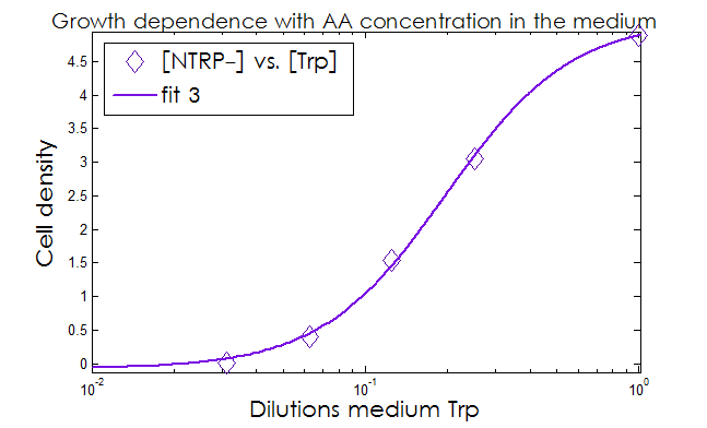
| - | + | *The '''Kaa''' found in the equations are related to the concentration of AAs in the medium required to reach half the maximum rate of growth. Curves of OD600 vs [AA](t=0) were measured experimentally for each amino acid and the data fitted to a Hill equation (6) using MATLAB’s TOOLBOX: Curve Fitting Tool. | |
| + | [[File:Bsas2012-modeling-eqfit.png|200px]](6) | ||
| - | + | This data from [[Team:Buenos_Aires/Results/Strains#Growth dependence on the Trp and His concentrations | experimental results]] and the best fit obtained for each are shown below in Figure 2. | |
| - | + | [[File:Bsas2012-modeling-fig_aux1.png]] | |
| + | [[File:Bsas2012-modeling-fig_aux2.png]] | ||
| + | Figure 2. Single strain culture density after over night growth vs the initial concentration of AA in the medium (dilutions 1:X). | ||
| + | The best fit to the data is also shown. | ||
| + | The values taken from the fits are | ||
| - | + | His- : | |
| + | K_dil = 0.2255 | ||
| + | n = 1.52 | ||
| + | R-square: 0.997 | ||
| - | + | Trp- : | |
| + | K_dil = 0.0469 | ||
| + | n = 1.895 | ||
| + | R-square: 0.998 | ||
| - | |||
| - | |||
| - | |||
| - | |||
| - | |||
| - | |||
| - | |||
| - | |||
| - | |||
| - | |||
| - | |||
| - | |||
| - | |||
| - | |||
| - | |||
| - | |||
| - | |||
| - | |||
| - | |||
| - | |||
| - | |||
| - | |||
| - | |||
| - | |||
| - | |||
| - | |||
| - | |||
| - | |||
| - | |||
| - | |||
| - | |||
| - | |||
| - | |||
| - | |||
| - | |||
| - | |||
| - | |||
| - | |||
| - | |||
| - | |||
| - | |||
| - | |||
| - | |||
| - | |||
| - | |||
| - | |||
| - | |||
| - | |||
| - | |||
| - | |||
| - | |||
| - | |||
| - | |||
| - | |||
| - | |||
| - | |||
| - | |||
| - | The | + | The results were then converted to the units chosen for the simulations. |
| - | [ | + | K = K_dil * [AA 1x] * Navog / (Molar mass AA) |
| - | + | where [AA 1x] = 0.02 mg/ml is the concentration of the AA (His or Trp) in the 1x medium and Navog is Avogadro's number. We get | |
| - | == | + | *K trp= .0469* 5.88e16 AA / ml = 2.76e15 molecules/ml |
| - | + | ||
| - | + | *K his= 0.2255* 7.8e16 AA / ml = 1.76e16 molecules /ml | |
| - | + | The competition within a strain and with the other were taken as equal. The system's general ''carrying capacity'' considered in the model is the one often used here, in a lab that works with these yeast strains: | |
| - | + | ||
| - | + | **Cc= 3e7 cell/ml. | |
| - | |||
| + | *The death rate was taken between 3 and 7 days. | ||
| - | |||
| - | The | + | *The rate of “production and export” was given an upper bound value (P_MAX) of 1% of the maximum estimated number of protein elongation events (peptidil transferase reactions) for a yeast cell per hour. That is, if all the biosynthetic capacity of the cell was used to create the AA rich exportation peptide, the export rate would equal P_MAX. Of course this is not possible because the cell has to do many other things, therefore we considered 1% of P_MAX as a reasonable upper bound for '''p'''. |
| + | From [http://www.biomedcentral.com/1752-0509/2/87| von der Haar 2008] we get an estimate for the total number of elongation events (peptidil transferase reactions): 6e6 1 / cell sec [ ] | ||
| - | + | * P_MAX = 2.16e8 1/ cell hour | |
| - | + | ||
| - | + | These parameters will be regulated in the simulation by ε and '''p''', to alter the fraction between populations. | |
| - | + | *p trp = '''p'''* '''ε'''*2.16e8 AA / cell hour | |
| - | + | *p his = '''p'''*2.16e8 AA / cell hour | |
| - | + | where '''p''' < 1 controls the fraction of the P_MAX value and ε the ratio between the export of each amino acid. | |
| - | |||
| - | + | '''d''' is the total number of amino acids in a yeast cell –same as the ones needed to create a daughter -per cell: | |
| - | + | ||
| - | + | ||
| - | + | '''d''' = # A.A. per cell = (mass of protein per yeast cell ) * relative abundance of AA * Navog / AA's molar mass. | |
| - | + | *d trp= 2.630e7 AA / cell | |
| + | *d his= 6.348e8 AA / cell | ||
| - | [ | + | ==Numerical Simulations== |
| - | + | :Initially we relied on numerical simulations (NS) performed with [http://www.mathworks.com/products/matlab/| MATLAB] to explore possible behaviors of the model, ODEs rarely have solutions that can be expressed in a closed form. | |
| - | + | :To run the simulations all that is left is to choose values {p, ε, initial conditions}. | |
| - | + | * Since this is merely a framewok we have taken values '''p''' from a log scale from -3 to 1. | |
| + | * '''ε''' was ranged from 0.0001 to 4; which varies the fraction of each population from 10% to 90%. | ||
| + | * Cells initial concentration (i.c.c.): dilutions from 1:10000 to 10x of the carrying capacity (Cc). | ||
| + | * Amino acids (AA) initial concentration: null, unless stated otherwise. | ||
| - | + | == Die or thrive?== | |
| + | :Some basic properties were observed by simplifying the system; we wanted to check that our model was sound. We considered a "symmetric interaction" in which both secretion rates and amino acid requirement were equivalent. | ||
| - | + | [[File:bsas2012-modeling-eq6.png]](7) | |
| - | + | where we can define | |
| - | + | [[File:bsas2012-modeling-eq7.png]] (8) | |
| - | + | :This parameter λ has an intuitive interpretation. The ratio '''d'''/'''p''' is the time it takes a cell to export enough AA for a cell of the other strain to build a daughter. On the other hand, 1/death is the average life span of a cell. Therefore λ is the ratio between the "life span" of a cell and the time it takes to export sufficient AA to build a cell, thus λ represents the amount of cells that can be constructed with the AA secreted by a cell in its lifetime. If this value is grated than one (λ > 1) the culture grows, otherwise it dies (This is completely analogous to the "force of infection" as defined in epidemiology). | |
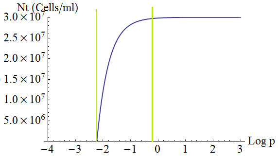
| - | + | :Keeping '''d''' and '''death''' constant, the total steady state number of cells in the culture depends on the secretion rate '''p''' as shown in the following figure 3. There is a threshold value p given by λ=1; with lower values the culture dies. | |
| - | + | ||
| - | + | ||
| - | + | [[File:bsas2012-modeling-fig3revised.png]] | |
| - | + | Figure 3. Total number of cells in the mix vs the strengh '''p''' of the production and export of AAs for a set of parameters Cc,d, death. | |
| - | |||
| - | |||
| - | + | :Another condition is related to extra-cellular concentration of amino acids. Looking at the equations for the evolution of the AA in the model, we can identify the parameter δ as follows | |
| - | + | [[File:bsas2012-modeling-eq8.png]](9) | |
| - | + | ||
| - | [[File:bsas2012-modeling- | + | |
| - | + | ||
| - | + | : As before, the ratio '''√(da db)/√(pa pb)''' is the average time required for a cell to export enough AA to construct another cell. '''1/kmax''' is the time it takes a cell to replicate in optimal growth conditions. δ can be interpret as the amount of cells that can be made with the material secreted a by a single cell before it divides (in optimal conditions). If δ > 1 the amount of nutrients produced exceeds the consumption, the medium gets saturated with AA and the regulation fails. So the system is auto-regulated only if δ < 1. | |
| - | + | :Combining these two conditions (λ > 1 and δ < 1), we conclude that the production rate has to be in a defined region for the system to work. To low and the culture dies out, to big and it gets out of control. | |
| - | + | ||
| - | == | + | == Parameter Space and Solutions == |
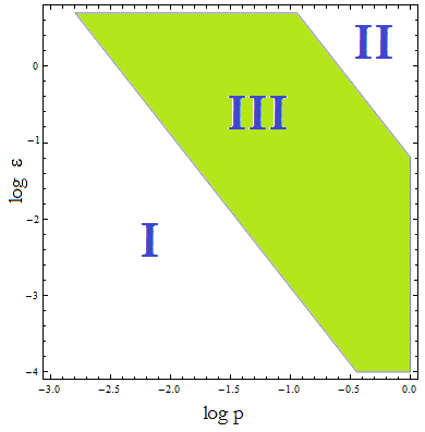
| + | :Uniting the conditions for λ and δ we see that in general '''p''' and ε must be bound for our solution to make sense (i.e. all concentrations > 0): | ||
| - | + | [[File:bsas2012-modeling-eq14.png]](10) | |
| - | |||
| - | + | [[File:bsas2012-modeling-fig3.png]] | |
| + | Figure 4. Regions in the parameter space that present different types of solutions. Only in Region III the system works as intended. | ||
| - | |||
| - | + | :Now, let's classify these regions numerically to see whether the ideas we just presented are supported. Taking random values from each region we found that all four variables are always positive, but each region is associated with a different kind of solution. The conditions shape the behavior and not the existence of a solution. | |
| - | + | :Taking AA(t=0)=0: | |
| - | + | ::I. The culture doesn't grow, it decays with varying velocities for any initial concentration of cells (i.c.c.). This is consistent with solution 1, where Nt= 0 as t → ∞. This is the λ < 1 case. | |
| - | |||
| - | + | ::II. The extracellular AA concentration keeps growing and the medium gets saturated. The culture reaches equilibrium for every i.c.c. no matter how low, but there is no regulation of the composition of the culture. This is the δ > 1 case. | |
| - | + | ::The growth rate tends to the theoretical 90 min and the AA dependence disappears from the equations for each population. Remarkably the fraction of each strain is still independent of the i.c.c. | |
| - | |||
| - | + | ::III. The four variables reach SS. The mole fraction is solely dependent on ε according to the formula on equation (5). The total population of the community (Nt) is the same as in Region II. | |
| - | + | ::'''This is the region where the auxotrophy leads to regulation of the community.''' However the culture doesn’t grow for all i.c.c. – will get back to this point shortly. | |
| - | == | + | ===Conclusions=== |
| + | ::Some conclusions we've drawn from these numerical simulations: | ||
| - | We' | + | # We had postulated that the solution doesn't hold in region II and expected a dramatic change in the system’s behavior. However there is a smooth transition between regions II and III. For a fixed ε we can go from region III to region II by increasing '''p'''. Once we cross the threshold we notice that the total population of cells (Nt) doeen't vary from one region to the next. Though the AA continues to grow over time (and accumulate) it does so slowly; more so than we'd expect for a vertical asymptote. |
| + | # More so, the formula (5) is a good approximation for the fraction of each strain in the region II close to the limit with region III; the difference between the two increases gradually as '''p''' gets further away from this threshold value. The formula is not true in II; thus regulation fails. | ||
| + | # There is no dramatic change caused by the asymptote, in fact the two regions can't be distinguished experimentally through a strain's fraction measurement in each side of the frontier; so small is the difference between the values across. | ||
| + | # Taking into account that the threshold is based on estimations; perhaps is safer to choose points well inside Region III to ensure proper regulation. This has a cost, for a fixed percentage the production and export of AAs is now lower and the dynamic of the culture slower. | ||
| - | + | :The original purpose of this analysis was to undertand '''under which initial conditions do the populations thrive or die'''. This has to be analyzed in terms of Figure 4, not merely the conditions for λ. | |
| - | + | ||
| - | + | ||
| - | + | ||
| - | + | ||
| - | + | ||
| - | + | ||
| - | + | ||
| - | + | ||
| - | + | ||
| - | + | ||
| - | + | ||
| - | + | ||
| - | + | ||
| - | + | ||
| - | + | ||
| - | + | ||
| - | + | ||
| + | :We noticed that the culture's survival in region III also depends on the values of '''Kaa''', even though is not explicit in any formula so far. Remember that '''Kaa''' is the concentration of an AA in the medium required for half maximal growth rate. For a fixed value of '''Kaa''' there is a critical initial concentration of cells below which the culture doesn't prosper. This effect is important when the percentage desired is extreme (close 100%), where the '''p''' value required for the strain gets really low. | ||
| + | :This is reasonable considering that another time scale is introduced. Not only have the cells to produce and absorb the required amounts of AA before they die, they also need to modify the AA concentration of the medium. The cells must produce enough amino acids so that the concentration of AA approximates '''Kaa'', before the original cells die out. If the initial cell density is to low, this won't happen. | ||
| - | |||
| - | + | == Lag Time == | |
| - | + | {| | |
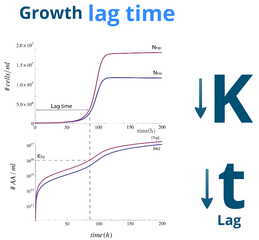
| + | |Let's finally look at some numerical simulations to see how the system evolves in time. We present a sample simulation with parameters from Region III to the rigth. There's a new characeristic that our previous analysis didn't show: the system reaches the desired steady state, however there will be significant lag phase. | ||
| - | + | We found numerically that it's related to time it takes for the Amino Acids in the medium to reach a certain concentration; one similar to the parameters '''Kaa''' and '''Kbb''' respectively. To this effect we note that it's possible to reduce this ''lag time'' by | |
| + | *Using higher initial concentration for each population. | ||
| - | * | + | *Lowering parameters '''Kaa''' and '''Kbb'''. |
| + | Given the relationship between these parameters and the AA absortion rates, we deviced a way to facilitate absortion. | ||
| + | We decided to work with | ||
| - | + | '''Troyan Peptides''' | |
| + | | | ||
| + | [[File:timeevol.jpg|350px]] | ||
| + | |- | ||
| + | |This lag time was quantified using the slowest strain's third cell division as a lag time. | ||
| - | + | The unit of the color scale is hours, it's clear than for lower initial concentrations and export rates | |
| - | + | | | |
| - | + | [[File:BsAs2012_11LagK.jpg.jpg|350px]] | |
| - | + | | | |
| - | + | |} | |
| - | + | ||
| - | + | ||
| - | + | ||
| - | + | ||
| - | + | ||
| - | + | ||
| - | + | ||
| - | + | ||
| - | + | ||
| - | + | ||
| - | + | ||
| - | + | ||
| - | + | ||
| - | + | ||
| - | + | ||
| - | + | ||
| - | + | ||
| - | + | ||
| - | + | ||
| - | + | ||
| - | + | ||
| - | + | ||
| - | + | ||
| - | + | ||
| - | + | ||
| - | + | ||
| - | + | ||
| - | + | ||
| - | + | ||
| - | + | ||
| - | + | ||
| - | + | ||
| - | + | ||
| - | + | ||
Latest revision as of 03:13, 27 October 2012

Contents |
Modeling a synthetic ecology
To gain insight into the behavior of our crossfeeding design, to understand which parameters of the system are important, and to study the feasibility of the project, we decided to implement a model of the system. We found this interesting per se, as the model we need is that of a microbial community and ecology.
The mathematical modeling of ecological system is an active field of research with a very rich and interesting history; from the works of Lotka and Volterra, who modeled predator-prey dynamics with ordinary differential equations, to Robert May’s chaotic logistic maps. In fact a lot of synthetic systems of interacting bacteria created in recent years were used to study these sort of models.
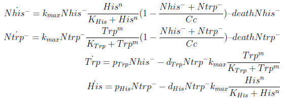
The crossfeeding model
In the crossfeeding design, each strain produces and releases to the medium an aminoacid the other strain(s) need to grow. The growth rate of each strain depends on the aminoacid (AA) concentration of those AA it can’t produce. In turn these concentrations depend on the abundance of the other strains. Therefore the growth of the strains is interdependent.
For simplicity and to be consistent with the experimental work, we decided to model two interacting strains, one that produces tryptophan (Trp) but requires histidine (His), and another that produces His but requires Trp.
We decided to use ordinary differential equations to model the system. This is a normal approach when studying population dynamics of this kind.
The model has four variables:
- [Nhis-] : the concentration of histidine dependent (Trp producing) yeast cells, in cells per ml
- [Ntrp-] : the total amount of tryptophan dependent (His producing) yeast cells, in cell per ml
- [his]: the concentration of histidine in the medium, in molecules per ml
- [trp]: the concentration of tryptophan in the medium, in molecules per ml.
To build the model we did the following assumptions:
- The growth rate of each strain depends on the concentration in the medium of the AA they can’t produce. As the concentration of this AA in the medium increases, so does the growth rate of the strain, until it settles at the growth rate observed in optimal conditions (doubling time of 90 min for yeast).
- There is a maximal density of cells the medium can support (carrying capacity)
- Each cell has a fixed probability of dying per time interval
- Each cell releases to the medium the AA it produces at a fixed rate
- Each strain only consumes the AA it doesn't produce
- The system reaches steady state.
In the equation for the temporal evolution of each population we take the growth rate as a Hill function of the amount of AA to which the strain is auxotrophic (it can't produce). The function captures the increase of the growth rate with the relevant AA concentration, until it reaches a plateau at the maximal growth rate, that corresponds to a doubling time of 90 minutes (doubling time = ln(2)/kmax). These functions are of the form
where Kaa is the effective concentration of AA at which half maximal growth rate is obtained, and l is the Hill coefficient, that describes how "steep" the curve is.
The term (1-(Nhis+Ntrp)/Cc) of the model accounts for other factors, not explicit in our model that can limit the concentration of cells in a given volume (carrying capacity), enabling the population to reach equilibrium. We included a term related to cell death (- death Ntrp), which is makes biologically sense (cell do die) and is critical for a correct behavior of the model.
The terms in the equations for the evolution of each [AA] in the medium are the fluxes of AA entering and leaving the medium. The first term (Ptrp*Nhis-) is a measure of the AA produced and exported in the form of peptides by a cell, for example the rate of tryptophan secretion by the histidine dependent cell.
The second term is the flux leaving the medium and entering the auxotrophic cells. Each cell has a more or less fixed amount of each amino acid, which we call d. If a cell is to replicate itself and cannot produce and amino acid, it will have to absorb it from the medium. Therefore the flux of AA entering the cell, is d divided by the doubling time τ (the time it takes to "construct" a new cell). One of the hypotheses built into our model is that τ will vary greatly with the concentration of nutrients available. We've used
The amount of AA entering the cells that produce it was considered negligible. This means that a cell that produces Trp doesn't import it from the medium in significant quantities. This is likely to hold when AA concentrations are limiting.
Steady State Solution
The 4 equations in the model were equaled to zero and the non-linear algebraic system solved using [http://www.wolfram.com/mathematica/ Mathematica] to find their equilibrium values.
Here we change the notation a little bit to two generic strains a and b where population Na produces amino acid a and requires b, and population Nb produces b and requires a. We are interested in the value of the cell populations in equilibrium, or more importantly the fraction of each population in steady state. Thus a change was made to more convenient variables: the sum of both population and a strain's fraction.
Nt = Na + Nb
Xa = Na / Nt
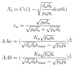
Only 3 fixed points were found for the system (See Appendix). There are some solutions for which it isn't true that the four variables reach a steady state (SS) or equilibrium. There are initial conditions for which the AA concentrations will not stop growing! So caution is required when assuming steady state.
- In the first solution we found the culture doesn't thrive, for example because one strain was missing or the initial density was to low.
- The second one has no biological relevance since it yields negative concentrations for the Amino Acids.
- The third one is the significant one (see equations below). However for some parameters the concentrations of Nt and AA can be negative, therefore restricting the parameter space in which the model works.
Regulation
Note that the fraction of each strain in the community is a function of the AA secretion rates (pa and pb) and the amount of AA required to "construct" a cell (da and db).
For positive values of d and p the range of the function is (0; 1), consistent with what we expect for a fraction.
The fraction of each strain in the culture in equilibrium are regulated by the production and export of each AA – represented in the model through pa and pb. These fractions are independent of initial conditions! This means that the system auto-regulates itself, as intended.
In fact we only need to control the ratio between these parameters to control the culture composition:
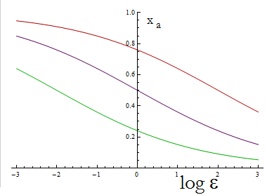
The next figure illustrates how the fraction Xa varies with the variable ε.
Figure 1. Fraction Xa as a fuction of the ratio of protein export for values of D=0.1,1,10 (in green, purple and red).
To programme the percentage we need a second set of biobricks that can sense an external stimulus and transduce this signal to modify ε. The range of percentages we can control is determined by the range of ε accessible with this second device and the ratio D that is set for any two A.A.
Parameters
The parameter estimation process is detailed in parameter selection
| Value | Units | |
| kmax | 0.4261 | 1/hr |
| K his | 2.588e16 | AA/ml |
| K trp | 1.041e16 | AA/ml |
| n his | 1.243 | |
| n trp | 1.636 | |
| Cc | 3.0 10^7 | cell/ml |
| death | 3 to 7 | days |
| p his | p 2.16e8 | AA/ cell hr |
| p trp | p ε 2.16e8 | AA/ cell hr |
| d his | 6.348e8 | AA/cell |
| d trp | 2.630e7 | AA/cell |
Table 1. Model parameters used for the simulations
Parameter selection
We estimatated values for all the parameter in the model, doing dedicated experiments or using values from the literature. This allowed to check the feasibility of the system.
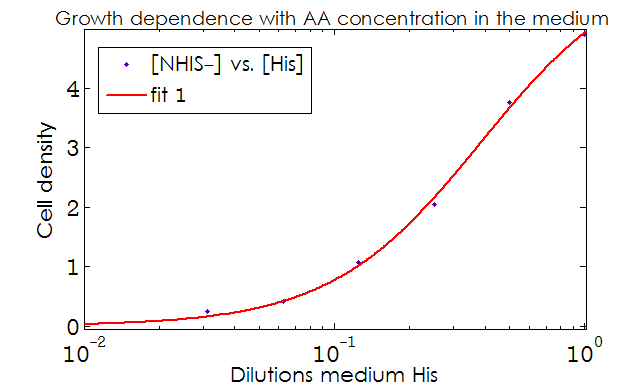
- The Kaa found in the equations are related to the concentration of AAs in the medium required to reach half the maximum rate of growth. Curves of OD600 vs [AA](t=0) were measured experimentally for each amino acid and the data fitted to a Hill equation (6) using MATLAB’s TOOLBOX: Curve Fitting Tool.
This data from experimental results and the best fit obtained for each are shown below in Figure 2.
Figure 2. Single strain culture density after over night growth vs the initial concentration of AA in the medium (dilutions 1:X).
The best fit to the data is also shown.
The values taken from the fits are
His- :
      K_dil =     0.2255
      n =          1.52
 R-square: 0.997
Trp- :
      K_dil =     0.0469
      n =          1.895
 R-square: 0.998
The results were then converted to the units chosen for the simulations.
K = K_dil * [AA 1x] * Navog / (Molar mass AA)
where [AA 1x] = 0.02 mg/ml is the concentration of the AA (His or Trp) in the 1x medium and Navog is Avogadro's number. We get
- K trp= .0469* 5.88e16 AA / ml = 2.76e15 molecules/ml
- K his= 0.2255* 7.8e16 AA / ml = 1.76e16 molecules /ml
The competition within a strain and with the other were taken as equal. The system's general carrying capacity considered in the model is the one often used here, in a lab that works with these yeast strains:
- Cc= 3e7 cell/ml.
- The death rate was taken between 3 and 7 days.
- The rate of “production and export” was given an upper bound value (P_MAX) of 1% of the maximum estimated number of protein elongation events (peptidil transferase reactions) for a yeast cell per hour. That is, if all the biosynthetic capacity of the cell was used to create the AA rich exportation peptide, the export rate would equal P_MAX. Of course this is not possible because the cell has to do many other things, therefore we considered 1% of P_MAX as a reasonable upper bound for p.
From [http://www.biomedcentral.com/1752-0509/2/87| von der Haar 2008] we get an estimate for the total number of elongation events (peptidil transferase reactions): 6e6 1 / cell sec [ ]
- P_MAX = 2.16e8 1/ cell hour
These parameters will be regulated in the simulation by ε and p, to alter the fraction between populations.
- p trp = p* ε*2.16e8 AA / cell hour
- p his = p*2.16e8 AA / cell hour
where p < 1 controls the fraction of the P_MAX value and ε the ratio between the export of each amino acid.
d is the total number of amino acids in a yeast cell –same as the ones needed to create a daughter -per cell:
d = # A.A. per cell = (mass of protein per yeast cell ) * relative abundance of AA * Navog / AA's molar mass.
- d trp= 2.630e7 AA / cell
- d his= 6.348e8 AA / cell
Numerical Simulations
- Initially we relied on numerical simulations (NS) performed with [http://www.mathworks.com/products/matlab/| MATLAB] to explore possible behaviors of the model, ODEs rarely have solutions that can be expressed in a closed form.
- To run the simulations all that is left is to choose values {p, ε, initial conditions}.
- Since this is merely a framewok we have taken values p from a log scale from -3 to 1.
- ε was ranged from 0.0001 to 4; which varies the fraction of each population from 10% to 90%.
- Cells initial concentration (i.c.c.): dilutions from 1:10000 to 10x of the carrying capacity (Cc).
- Amino acids (AA) initial concentration: null, unless stated otherwise.
Die or thrive?
- Some basic properties were observed by simplifying the system; we wanted to check that our model was sound. We considered a "symmetric interaction" in which both secretion rates and amino acid requirement were equivalent.
where we can define
- This parameter λ has an intuitive interpretation. The ratio d/p is the time it takes a cell to export enough AA for a cell of the other strain to build a daughter. On the other hand, 1/death is the average life span of a cell. Therefore λ is the ratio between the "life span" of a cell and the time it takes to export sufficient AA to build a cell, thus λ represents the amount of cells that can be constructed with the AA secreted by a cell in its lifetime. If this value is grated than one (λ > 1) the culture grows, otherwise it dies (This is completely analogous to the "force of infection" as defined in epidemiology).
- Keeping d and death constant, the total steady state number of cells in the culture depends on the secretion rate p as shown in the following figure 3. There is a threshold value p given by λ=1; with lower values the culture dies.
Figure 3. Total number of cells in the mix vs the strengh p of the production and export of AAs for a set of parameters Cc,d, death.
- Another condition is related to extra-cellular concentration of amino acids. Looking at the equations for the evolution of the AA in the model, we can identify the parameter δ as follows
- As before, the ratio √(da db)/√(pa pb) is the average time required for a cell to export enough AA to construct another cell. 1/kmax is the time it takes a cell to replicate in optimal growth conditions. δ can be interpret as the amount of cells that can be made with the material secreted a by a single cell before it divides (in optimal conditions). If δ > 1 the amount of nutrients produced exceeds the consumption, the medium gets saturated with AA and the regulation fails. So the system is auto-regulated only if δ < 1.
- Combining these two conditions (λ > 1 and δ < 1), we conclude that the production rate has to be in a defined region for the system to work. To low and the culture dies out, to big and it gets out of control.
Parameter Space and Solutions
- Uniting the conditions for λ and δ we see that in general p and ε must be bound for our solution to make sense (i.e. all concentrations > 0):
Figure 4. Regions in the parameter space that present different types of solutions. Only in Region III the system works as intended.
- Now, let's classify these regions numerically to see whether the ideas we just presented are supported. Taking random values from each region we found that all four variables are always positive, but each region is associated with a different kind of solution. The conditions shape the behavior and not the existence of a solution.
- Taking AA(t=0)=0:
- I. The culture doesn't grow, it decays with varying velocities for any initial concentration of cells (i.c.c.). This is consistent with solution 1, where Nt= 0 as t → ∞. This is the λ < 1 case.
- II. The extracellular AA concentration keeps growing and the medium gets saturated. The culture reaches equilibrium for every i.c.c. no matter how low, but there is no regulation of the composition of the culture. This is the δ > 1 case.
- The growth rate tends to the theoretical 90 min and the AA dependence disappears from the equations for each population. Remarkably the fraction of each strain is still independent of the i.c.c.
- III. The four variables reach SS. The mole fraction is solely dependent on ε according to the formula on equation (5). The total population of the community (Nt) is the same as in Region II.
- This is the region where the auxotrophy leads to regulation of the community. However the culture doesn’t grow for all i.c.c. – will get back to this point shortly.
Conclusions
- Some conclusions we've drawn from these numerical simulations:
- We had postulated that the solution doesn't hold in region II and expected a dramatic change in the system’s behavior. However there is a smooth transition between regions II and III. For a fixed ε we can go from region III to region II by increasing p. Once we cross the threshold we notice that the total population of cells (Nt) doeen't vary from one region to the next. Though the AA continues to grow over time (and accumulate) it does so slowly; more so than we'd expect for a vertical asymptote.
- More so, the formula (5) is a good approximation for the fraction of each strain in the region II close to the limit with region III; the difference between the two increases gradually as p gets further away from this threshold value. The formula is not true in II; thus regulation fails.
- There is no dramatic change caused by the asymptote, in fact the two regions can't be distinguished experimentally through a strain's fraction measurement in each side of the frontier; so small is the difference between the values across.
- Taking into account that the threshold is based on estimations; perhaps is safer to choose points well inside Region III to ensure proper regulation. This has a cost, for a fixed percentage the production and export of AAs is now lower and the dynamic of the culture slower.
- The original purpose of this analysis was to undertand under which initial conditions do the populations thrive or die. This has to be analyzed in terms of Figure 4, not merely the conditions for λ.
- We noticed that the culture's survival in region III also depends on the values of Kaa, even though is not explicit in any formula so far. Remember that Kaa is the concentration of an AA in the medium required for half maximal growth rate. For a fixed value of Kaa there is a critical initial concentration of cells below which the culture doesn't prosper. This effect is important when the percentage desired is extreme (close 100%), where the p value required for the strain gets really low.
- This is reasonable considering that another time scale is introduced. Not only have the cells to produce and absorb the required amounts of AA before they die, they also need to modify the AA concentration of the medium. The cells must produce enough amino acids so that the concentration of AA approximates 'Kaa, before the original cells die out. If the initial cell density is to low, this won't happen.
Lag Time
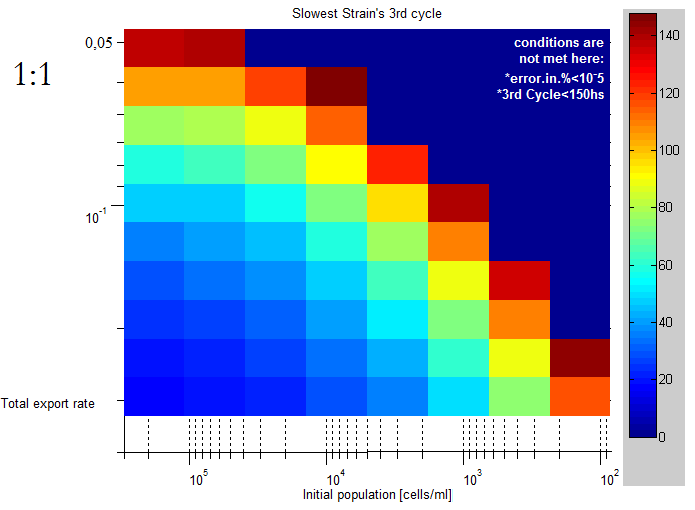
| Let's finally look at some numerical simulations to see how the system evolves in time. We present a sample simulation with parameters from Region III to the rigth. There's a new characeristic that our previous analysis didn't show: the system reaches the desired steady state, however there will be significant lag phase.
We found numerically that it's related to time it takes for the Amino Acids in the medium to reach a certain concentration; one similar to the parameters Kaa and Kbb respectively. To this effect we note that it's possible to reduce this lag time by
Given the relationship between these parameters and the AA absortion rates, we deviced a way to facilitate absortion. We decided to work with Troyan Peptides | ||
| This lag time was quantified using the slowest strain's third cell division as a lag time.
The unit of the color scale is hours, it's clear than for lower initial concentrations and export rates |
 "
"
