Modeling methods

• Introduction
  
• Cooperativity
• Deterministic modeling
• Stochastic modeling
• Quantitative model and stability analysis
• C#Sim - algorithmic modeling
• Source code

Introduction

In order to examine (i.e. simulate) the proposed genetic switches in silico, different modeling approaches were used. First, a deterministic model based on the probabilistic interpretation of gene regulation was constructed for each type of a genetic switch. Next, a stochastic simulation was performed to take inherent stochastic dynamics of gene expression into account. To further verify the results obtained using these methods, we also developed a quantitative model that builds upon experimental data. Moreover, we developed a modeling algorithm to more explicitly simulate transcription factor binding, considering number of available binding sites and competitive binding. Each modeling approach is discussed in the following sections. We also discuss the notion of cooperativity in the context of bistability.

Cooperativity

It is often assumed that functional cooperativity (e.g. multimeric regulation) is required for bistability. However, it has been shown theoretically that bistability can emerge in systems without multimeric regulation, provided that at least one regulatory autoloop is present. (Widder et al., 2009). Furthermore, in silico analysis has shown the existence of bistable architectures without the transcription factor cooperativity typically associated with switch-like properties (Siegal-Gaskins et al., 2011). An essential feature of these proposed architectures was the competitive binding of two transcription factors to the promoter.

In terms of modeling, sigmoidal functions (characterizing the rate of change dP/dt) – arising from (Hill) exponents greater than one - are often equated with molecular cooperativity (the way the transcription factor binds to a promoter). However, as non-linearity and multi-stability can arise without assuming molecular cooperativity, it has been suggested that this is not an accurate proposition and that mathematical or functional cooperativity – referring to a sigmoidal function arising from system equations - should not automatically be interpreted as molecular cooperativity (Andrecut et al., 2011). One reason for this is that model equations represent a significant simplification of actual biological dynamics of gene expression, which include a large number of reactions not explicitly considered in modeling, such as reactions describing chromosome opening and transcription initiation.

For this reasons, we believe that sigmoidal behavior alone – arising in some of our models for transcription factors’ exponent values (non-linearity) greater than 1 - should not by default be interpreted as molecular cooperativity. Thus, in the context of modeling, with the term cooperativity we mean functional cooperativity greater than 1. Functional cooperativity equal to 1 is referred to as no cooperativity.

Indeed, in case of our positive feedback loop switch – which contains both competitive binding and regulatory autoloops - even deterministic models predict experimentally-verified bistability at low (i.e. close to 1; deterministic fractional occupancy model) or no (quantitative model) functional cooperativity. Our stochastic model of the positive feedback loop switch also predicts bistability is possible without cooperativity.

Deterministic modeling

Our deterministic models are based on fractional occupancy, a quantity which expresses the degree of saturation at the transcription factor binding site (Sauro, 2012). Fractional occupancy can be expressed as a ratio of active binding site states – i.e. states leading to gene expression – to all possible binding site states:

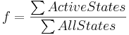
As such, it can be interpreted as a probability of a promoter being active, or a probability that transcription and/or translation will occur. Gene expression in our model, in turn, is proportional to this probability.

Two main possibilities are distinguished in our models depending on the type of the promoter. In case of a minimal promoter, binding of a transcriptional activator (leading to an active state) is required for transcription initiation. Other states – binding site being free or bound by a repressor - are considered inactive. In case of a constitutive promoter, binding of a transcriptional repressor leads to an inactive state, while unbound (or activator-bound) states are active, hence leading to gene expression.

We assumed large species concentrations compared to the number of available binding sites. We also assumed fast transitions between promoter states, i.e. transcription factor binding and unbinding occurs much faster than transcription/translation, which in this type of deterministic models are represented as a single step of protein production. Another simplification made was a representation of multiple repeats of a binding site as a single binding site (e.g. a specific TAL-A:KRAB binding site may in reality have 10 repeats, while in our models it is represented as a single site). As the purpose of our deterministic models is to provide an approximate, basic characterization of the proposed logic, we consider these simplifications acceptable. Other models, such as C#Sim models (described later), try to formalize some of these aspects in more detail.

The mathematical framework which describes protein production and into which we incorporate fractional occupancy is represented as a set of ordinary differential equations (ODEs) of the form:

and is roughly based on a framework proposed in (Kaern et al., 2005). Here:

• [Protein] is protein concentration at a given time;
• k is a constant specifying protein production rate in case of an active promoter.
• kb is a constant specifying the amount of leaky gene expression, meaning protein production that takes place even in the case of inactive (i.e. repressed constitutive or non-activated minimal) promoter.
• dg is a constant specifying protein degradation rate.
• P(active) is the probability of a promoter being in an active state – this probability is equal to fractional occupancy f.
• P(inactive) is the probability of a promoter being inactive and is equal to (1-f).

No specific quantitative data describing e.g. transcription, translation or degradation rates of TAL effectors was available to us. For this reason, the parameter values (specifying e.g production or degradation rates) in our models were assumed based on commonly accepted propositions, such as that production (i.e. transcription and translation) rates of proteins are (usually) higher than their degradation rates. Parameter values that were used in our simulations should hence only be considered in relative terms (e.g. as protein production to degradation ratios). We also assumed parameter symmetry of different TAL effectors used (TAL-A and TAL-B), because we did not expect that one would have e.g. a production rate significantly higher than the other.

All deterministic models were implemented in MATLAB.

Stochastic modeling

Gene expression is an inherently stochastic process and deterministic simulation is often not satisfactory. The required conditions for the two approaches to be similar are large system size (high mRNA and protein numbers) and fast promoter kinetics (Kaern et al., 2005), but these conditions are not always met. Furthermore, stochastic models can capture the individuality of single cells, as opposed to deterministic models that can only predict the average behavior of a cell population (Kaern et al., 2003). For this reason we performed stochastic simulations of the proposed genetic switches. Our results were obtained using SGN Sim, a stochastic genetic networks simulator (Ribeiro et al., 2007) based on stochastic simulation algorithm (SSA).

Competitive binding between an activator and a repressor exists in our positive feedback loop switch. This can lead to three major minimal promoter states: the promoter being free (i. e. unbound - neither an activator nor a repressor is bound, zero activation is present), bound by a repressor or bound by an activator. When minimal promoter is unbound, only leaky expression occurs. If bound by an activator, this causes high activated expression levels. Bound repressor causes the expression levels to drop even below the ones achieved for the unbound (non-activated) state.

Our deterministic models made no clear distinction between free (unbound) minimal promoter state and a repressor-bound state – in both cases inactive promoter state was assumed, leading to only leaky expression. In our stochastic models we improved this by introducing different expression levels for all three states, achieving a more realistic formalization.

Quantitative model and stability analysis

Based on experimental data we constructed what we refer to as a quantitative model. Please see Quantitative and stability model for details. To get a better idea of the functioning of the model, an interactive web application was developed.

C#Sim - algorithmic modeling

We developed a new modeling algorithm called C#Sim. The main purpose of this was:

• to explicitly model a limited number of binding site repeats;
• to explicitly model competitive binding of activators and repressors;
• to construct a new modeling approach that incorporates stochasticity of gene expression into an otherwise deterministic approach.

The assumptions made here were similar to that of deterministic modeling. First, we assumed that high concentrations of mRNA and proteins existed compared to the number of available binding sites that transcription factors could bind to. Second, we assumed that binding of transcription factors to binding sites was much faster than transcription and translation.

A feature of C#Sim is that it operates with discrete numbers – at each step of the simulation, mRNA and protein amounts are non-negative integers. Each mRNA and protein molecule is represented as an independent entity – or object - defined by its parameters and interactions. An object-oriented programming approach was used to achieve this. At the moment, C#Sim supports the following entity types, implemented as classes:

mRNA
Parameters: birth time (integer) – tells at what simulation step this mRNA entity was created (transcribed); used for modeling transcription-translation delay; alive (true/false) – tells if this mRNA is alive and subject to translation (true) or not.

Protein
Parameters: birth time (integer) – tells at what simulation step this protein entity was created (translated); alive (true/false) – tells if this protein is alive (true), e.g. it can function as a transcription factor.

Binding site
Parameters: capacity (integer) – the number of binding site repeats; each repeat can be bound by one protein entity; amount of bound activator (integer) – the number of activator entities bound to this binding site; amount of bound repressor (integer) – the number of repressor entities bound to this binding site.

Promoter

Parameters: promoter type – either minimal or constitutive; list of promoter binding sites; active mRNA transcription rate, which determines the number of mRNA entities to produce at each simulation step for activated promoter (in case of a minimal promoter) or non-repressed promoter (in case of a constitutive promoter); inactive (leaky) mRNA transcription rate, which determines the number of mRNA entities that can be produced even when the promoter is not activated (for minimal promoter), or when the promoter is repressed (for constitutive promoter); the amount of all repressors and activators bound to all promoter binding sites.

Gene
Parameters: gene's promoter; translation rate, describing the number of proteins produced per each transcribed alive mRNA entity at each simulation step; mRNA and protein degradation rate (i.e. the percentage of mRNA and protein degraded at each simulation step).

Note that the majority of these parameters are computed automatically, not specified by the user (programmer). The parameters specified by the user (when defining the network structure) are: binding sites' capacities, promoter types, list of promoter binding sites, active and inactive transcription rates, a promoter for each gene, translation rates and degradation rates. A delay between transcription and translation can also be specified.

Using these entities, a hierarchy of gene regulatory network can quickly be constructed. Furthermore, the approach is highly modular and extendible with new dynamics.

Other parameters also define the behavior of the mentioned entity types – they are listed and explained in more detail in the algorithm overview below.

Algorithm overview

C#Sim modeling consists of two major steps:

1. Define gene regulatory network structure as a series of related entities (objects): genes to transcribe and translate, promoters, binding sites and transcription factor binding interactions. Specify necessary parameters, such as production rates, degradation rates and promoter binding sites.
2. Specify the number of simulation steps. At each step of the simulation:
   1. (optional) introduce input signals and define their actions (e.g. introduce signal 1 at a specific time of the simulation and make it prevent transcription factor from binding);
   2. transcribe and translate genes; degrade (i.e. delete) a parameter-specified percentage of produced mRNA and proteins;
   3. bind existent transcription factor proteins to their target binding sites; considering binding site capacity (i.e. the number of binding site repeats), uniformly distribute transcription factors among target binding sites;
   4. execute the next simulation step.

Transcription factor binding

Each binding site is modeled as an individual entity. The algorithm, at each simulation step, uniformly distributes transcription factors among their target binding sites based on the amount of each transcription factor available. A binding site entity, B, is defined by the following parameters:

• capacity, C (i.e. the number of binding site repeats);
• the amount of bound activator, B_A (integer) – how many activator entities are bound to this binding site;
• the amount of bound repressor, B_R (integer) – how many repressor entities are bound to this binding site.

The sum of all repressors and activators bound to a binding site is never greater than that binding site capacity:

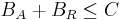
Let A be the amount of activator entities (objects) available for binding and R the amount of repressor entities available for binding. Activators and repressors that competitively bind to a binding site B distribute among the available binding site repeats (specified by capacity C) uniformly, with equal binding affinity, according to the following equations:

• if A+R < C, then:
  B_A = A
  B_R = R


• if A+R is greater or equal than C, then:

  

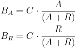
All values are non-negative integers, i.e. rounding is used to obtain final B_A and B_R values. These equations can easily be generalized for a non-competitive binding scenario, when only activators or only repressors bind – in the first case, R is set to 0 (i.e. only activator entities are available); in the second case, A is set to zero (i.e. only repressor entities are available).

For example, let 10 TAL-A binding site repeats exist, meaning TAL-A binding site capacity is equal to 10. TAL-A:KRAB and TAL-A:VP16 competitively bind for this binding site. Suppose that at a given time the available amount of each of these proteins is 100 units:

• TAL-A:KRAB = 100 units
• TAL-A:VP16 = 100 units

The amount of TAL-A:VP16 that will bind to the TAL-A binding site is:

meaning 5 binding site repeats will become bound by the TAL-A:VP16. Similarly the other 5 will become bound by the TAL-A:KRAB:

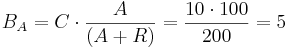
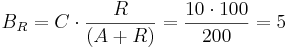
Thus a uniform distribution was achieved.

Bound proteins degrade in the same manner as the unbound proteins. It should be noted that with transcription and translation in the context of this algorithm we also mean mRNA and protein degradation.

Transcription

The following algorithm steps constitute transcription. For each gene to transcribe at each simulation step:

1. count the total amount of repressor and activator entities that are bound to all gene promoter binding sites:

   

   B_Ri is the amount of repressor bound at binding site i. B_Ai is the amount of activator bound at binding site i.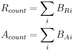


2. If the promoter is minimal, calculate the amount of mRNA to produce, N'_mRNA, in this simulation step:

   

   Here: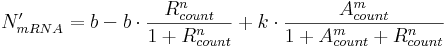
   • b is inactive (i.e. leaky) transcription rate, specifying mRNA production rate when no activators and no repressors are bound;
   • k is active (i.e activated) transcription rate and is typically much higher than b; it specifies mRNA production rate when activators are bound;
   • n and m are transcription factor exponents, specifying the degree of non-linearity.
   
   

   The structure of this equation is such because we distinguish between three major minimal promoter states:

   • free (unbound) state, meaning no repressor and no activator entities are bound to corresponding binding sites; in this case, N'_mRNA will be equal to b (leaky rate);
   • repressor-bound state, meaning only repressor is bound to corresponding binding sites; in this case, bound repressor can – because of the second term of the equation – decrease the basal rate and hence N'_mRNA;
   • activator-bound state, meaning only activator is bound; in this case, the second term of the equation will be equal to zero and (assuming k is much larger than b) N'_mRNA will be large, indicating activated transcription.

   When both activators and repressors are bound to binding sites, none of the three terms will be equal to zero (provided b and k are non-zero values). Because bound repressor count, R_count, occurs in two terms, while bound activator count, A_count, only occurs in one term, the effect of bound repressors on N'_mRNA will be more pronounced compared to the effect of bound activators. This way, a requirement for repression priority over activation (i.e. a small amount of bound repressor significantly reduces expression levels, despite bound activator) is met.



3. If the promoter is constitutive, calculate the amount of mRNA to produce, N'_mRNA, in this simulation step:

   

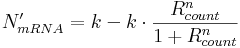
   With our switches in mind, only repressors can bind to constitutive promoter binding sites, hence the equation only has two terms. Here,

   • k is the active (non-repressed, constitutive) transcription rate, reached only when no repressor entities are bound;
   • n is an exponent specifying the degree of non-linearity.
   Repressor binding can thus decrease N'_mRNA.




4. Randomly increase or decrease calculated N'_mRNA – this way, stochasticity of transcription is taken into account (e.g. some bound transcription factor can unbind from the binding site). In this step, N'_mRNA is altered to a new value:

   

   where r is a random integer (uniform distribution is used) from the interval

   

   and t is a real-value parameter between 0 and 1 and specifies the intensity of transcription stochasticity. For our simulations, t was always equal to 0.45.



5. If N_mRNA was set to 0, make N_mRNA equal to leaky transcription rate parameter, b, with probability P_L (probability of leaky expression – equal to 90 % in our simulations). This probability is used to allow more control over the dynamics of leaky expression.


6. Transcribe (generate) N_mRNA mRNA entities (objects).


7. Degrade m % of mRNA available in the system.

Translation

The following algorithm steps constitute translation. For each existing mRNA entity, at each simulation step:

1. with a probability of P_T (we refer to this value as translation probability, or translation effectiveness), generate T_r protein entities, where T_r is the translation rate (equal to 1 in all our simulations); mRNA is only translated if the transcription-translation delay has elapsed;


2. degrade p % of proteins in the system.

Source code

Our modeling-related source code can be found here.

References

Andrecut M, Halley JD, Winkler DA, Huang S. (2011) A General Model for Binary Cell Fate Decision Gene Circuits with Degeneracy: Indeterminacy and Switch Behavior in the Absence of Cooperativity. PLoS ONE 6, e19358. doi:10.1371/journal.pone.0019358.

Kaern M, Blake WJ, Collins JJ. (2003) The engineering of gene regulatory networks. Annual Review of Biomedical Engineering. 5, 179-206.

Kaern M, Elston TC, Blake WJ, Collins JJ. (2005) Stochasticity in gene expression: from theories to phenotypes. Nature. 6, 451-464.

Ribeiro AS, Lloyd-Price J. (2007) SGN Sim, a Stochastic Genetic Networks Simulator. Bioinformatics. 23, 777-779.

Sauro HM. (2012) Enzyme Kinetics for Systems Biology. Future Skill Software.

Siegal-Gaskins D, Mejia-Guerra MK, Smith GD, Grotewold E. (2011) Emergence of Switch-Like Behavior in a Large Family of Simple Biochemical Networks. PLoS Comput Biol 7, e1002039. doi:10.1371/journal.pcbi.1002039.

Widder S, Macía J, Solé R. (2009) Monomeric Bistability and the Role of Autoloops in Gene Regulation. PLoS ONE 4, e5399. doi:10.1371/journal.pone.0005399.

---

Next: Deterministic model of the mutual repressor switch >>