Team:TU Munich/Modeling/Gal1 Promoter
From 2012.igem.org
(→Profile Likelihood) |
(→Joint Distribution) |
||
| Line 100: | Line 100: | ||
<div style="clear:both"> | <div style="clear:both"> | ||
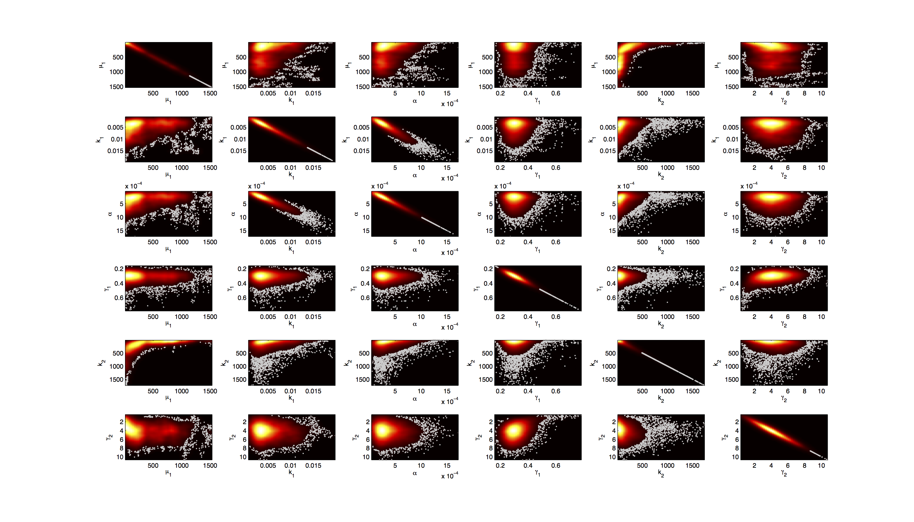
| - | For the smoothed histogram plot [http://www.mathworks.de/matlabcentral/fileexchange/13352-smoothhist2d | + | For the smoothed histogram plot smoothhist2d.m[http://www.mathworks.de/matlabcentral/fileexchange/13352-smoothhist2d] was used. The color indicates the density of samples. Black to dark red reflects a low density, yellow to white indicates a high density. Grey dots indicate samples identified as outliers by the script. |
For the scatter plot further thinning of 1:1000 was necessary for scatter.m to be able to process the data. | For the scatter plot further thinning of 1:1000 was necessary for scatter.m to be able to process the data. | ||
| - | On the diagonal the kernel density estimation script [http://www.mathworks.com/matlabcentral/fileexchange/14034-kernel-density-estimator | + | On the diagonal the kernel density estimation script kde.m[http://www.mathworks.com/matlabcentral/fileexchange/14034-kernel-density-estimator] was used to obtain a plot of the density. Here the color indicates the a-posterior probability of the respective sample. Low probabilities are mapped by blue to green color, High probabilities are mapped by yellow to red color. |
Mind that due to the nature of the the utilized scripts, the orientation of the Y-Axis is flipped when comparing the two plots. | Mind that due to the nature of the the utilized scripts, the orientation of the Y-Axis is flipped when comparing the two plots. | ||
Revision as of 14:49, 16 September 2012


Contents |
Gal1 Promoter
The Gal1 Promoter is the standard promoter for our pYES vector that is used in the expression of all ingredient pathways. As it is also part of the construct for the light switchable promoter, it is crucial to thoroughly characterize the kinetics of this promoter.
Model Specification
Model Equations
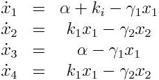
We used a two species approach for mRNA and Protein concentrations. x1 and x2 represent the mRNA and protein levels for the induced promoter and x3 and x4 the respective levels for the uninduced promoter.
As no analysis was done with several galactose concentrations hence the hill function that normally models the response to the concentration was replaced by a single factor to improve identifiability.
Parameters
| Name | Description | Prior? | Best fit | Unit |
| μ | Scaling factor | NO | 114.9 | - |
| ki | Induced transcription rate | YES | 0.006758 | mol/h |
| α | Leaky transcription rate | NO | 0.0004784 | mol/h |
| γ1 | mRNA degradation rate | YES | 0.2892 | 1/h |
| k2 | Protein synthesis rate | NO | 165.9 | mol/h |
| γ2 | Protein degradation rate | NO | 3.1874 | 1/h |
| σ1 | Standard deviation for measured data of induced cells | NO | 19.55 | - |
| σ2 | Standard deviation for measured data of noninduced cells | NO | 5.337 | - |
Data
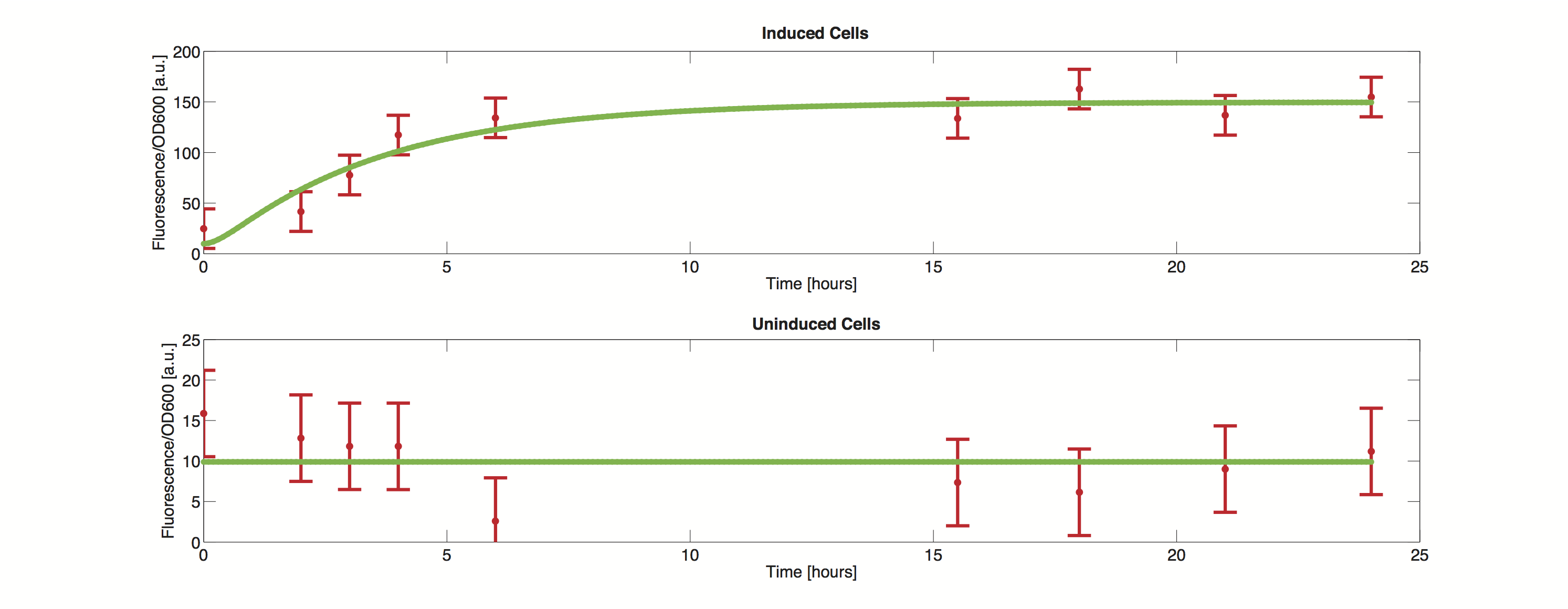
The methods utilized rely on a value for standard deviation, but only one experimental measurement was performed. Hence a value was infered during the optimization process. Thus the error bars in the plot do not reflect values from actual measurements but merely show how well the data can be approximated by the model.
Profile Likelihood
For the profile likelihood analysis, the scripts provided by the Systems Biology group from TU Eindhoven [1] were used and modified to our needs.
Markov Analysis
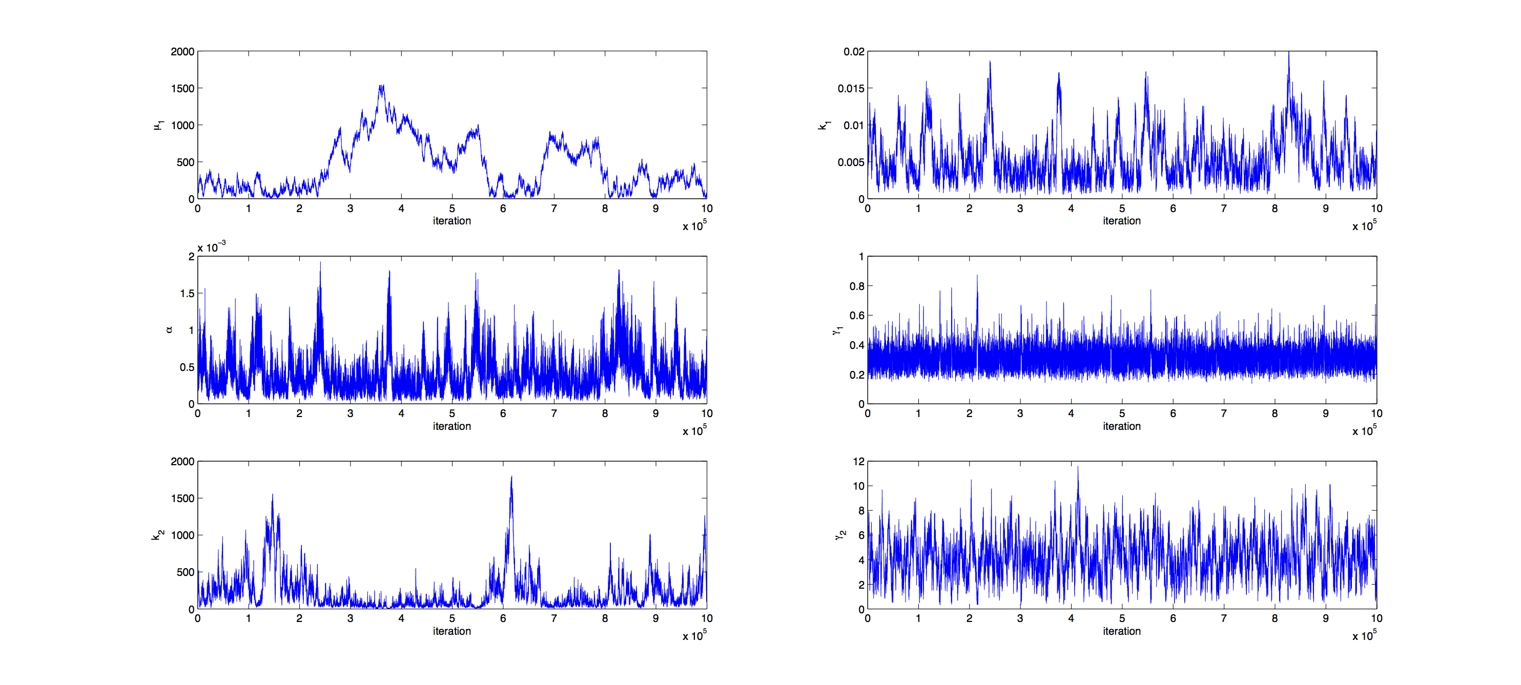
Analysis was performed with a Metropolis Hastings algorithm. 1000000 samples were generated and then thinned by a factor 1:100 to reduce correlation of the samples. The acceptance rate for the samples was 16% so a little below the target of 23%.
Joint Distribution
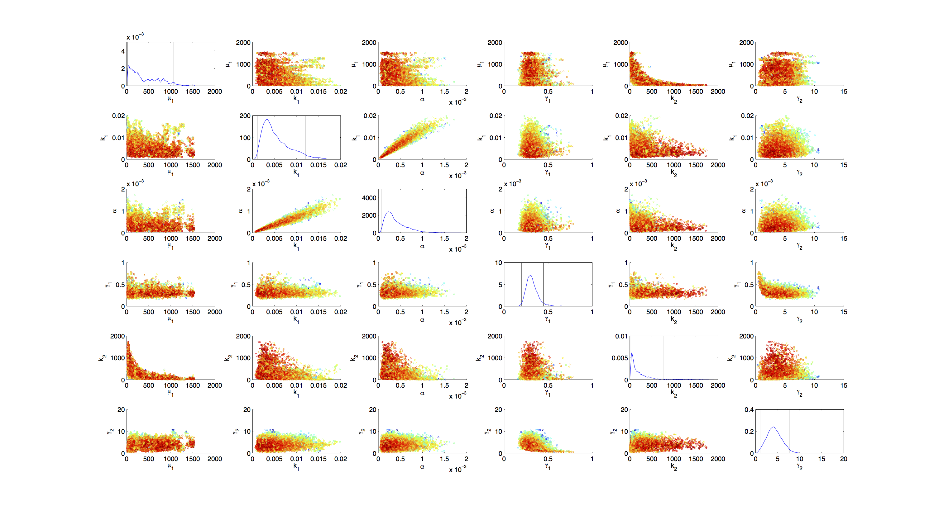
For the smoothed histogram plot smoothhist2d.m[2] was used. The color indicates the density of samples. Black to dark red reflects a low density, yellow to white indicates a high density. Grey dots indicate samples identified as outliers by the script.
For the scatter plot further thinning of 1:1000 was necessary for scatter.m to be able to process the data. On the diagonal the kernel density estimation script kde.m[3] was used to obtain a plot of the density. Here the color indicates the a-posterior probability of the respective sample. Low probabilities are mapped by blue to green color, High probabilities are mapped by yellow to red color.
Mind that due to the nature of the the utilized scripts, the orientation of the Y-Axis is flipped when comparing the two plots.
Credibility Intervals
As the Metropolis Hastings algorithm samples exactly from the target distribution, one can use the generated samples to find credibility intervals. The shown intervals are maximum density credibility intervals. They were obtained by computing the 1-α/2; and α/2 quantiles, with alpha being the missing percentage to 100%, that minimized the 1-norm of the distance between the two values.
| Param. | μ1 | k1 | α | γ1 | k2 | γ2 |
| 95% | [7.6525 , 203.2962] | [0.0011078 , 0.017724] | [8.0055e-05 , 0.001293] | [0.20397 , 0.45586] | [24.3219 , 954.8224] | [1.0073 , 7.3142] |
| 75% | [14.3725 , 116.5086] | [0.0020553 , 0.0089666] | [0.00012838 , 0.00064765] | [0.24028 , 0.3761] | [126.3764 , 646.5652] | [1.8417 , 5.5854] |
| 50% | [14.7945 , 73.2214] | [0.002091 , 0.0058511] | [0.00017481 , 0.00044449] | [0.25771 , 0.33486] | [327.0597 , 639.2103] | [2.4019 , 4.6641] |
Covariance
| Param. | μ1 | k1 | α | γ1 | k2 | γ2 |
| μ1 | 9.5206278866 | 0.0005577146 | 0.0000392198 | 0.0249444112 | 12.9374858110 | 0.2451232424 |
| k1 | 0.0005577146 | 0.0000000334 | 0.0000000023 | 0.0000014843 | 0.0007684788 | 0.0000145516 |
| α | 0.0000392198 | 0.0000000023 | 0.0000000001 | 0.0000001037 | 0.0000536326 | 0.0000010162 |
| γ1 | 0.0249444112 | 0.0000014843 | 0.0000001037 | 0.0000662780 | 0.0341311274 | 0.0006455975 |
| k2 | 12.9374858110 | 0.0007684788 | 0.0000536326 | 0.0341311274 | 17.7991401047 | 0.3367804890 |
| γ2 | 0.2451232424 | 0.0000145516 | 0.0000010162 | 0.0006455975 | 0.3367804890 | 0.0063804120 |
Sensitivity Analysis
Conclusion
== Reference ==
 "
"
