Team:TU Munich/Modeling/Gal1 Promoter
From 2012.igem.org


Contents |
Modeling: Gal1 Promoter
The Gal1 Promoter is the standard promoter for our pYES vector that is used in the expression of all ingredient pathways. As it is also part of the construct for the light switchable promoter, it is crucial to thoroughly characterize the kinetics of this promoter.
For details about the methods used see Team:TU_Munich/Modeling/Methods
Model Specification
Model Equations
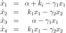
We used a two species approach for mRNA and Protein concentrations. x1 and x2 represent the mRNA and protein levels for the induced promoter and x3 and x4 the respective levels for the uninduced promoter.
As no analysis was done with several galactose concentrations hence the hill function that normally models the response to the concentration was replaced by a single factor to improve identifiability.
Parameters
| Name | Description | Prior? | Best fit | Unit |
| μ | Scaling factor for x2 and x4 when computing the difference to the data. Represents the fluorescence units per protein. | NO | 114.9 | - |
| ki | Induced transcription rate | YES | 0.006758 | mol/h |
| α | Leaky transcription rate | NO | 0.0004784 | mol/h |
| γ1 | mRNA degradation rate | YES | 0.2892 | 1/h |
| k2 | Protein synthesis rate | NO | 165.9 | mol/h |
| γ2 | Protein degradation rate | NO | 3.1874 | 1/h |
| σ1 | Standard deviation for measured data of induced cells | NO | 19.55 | - |
| σ2 | Standard deviation for measured data of noninduced cells | NO | 5.337 | - |
The best fit is in a-posterior sense where the logarithm of the a-posteriori was optimized using the Matlab script lsqnonlin. The script uses a Levenberg-Marquardt algorithm to find a minimum.
All fitted parameters are within realistic bounds.
The half life time of eGFP is a bit lower than expected. The literature states GFP should have a half-life time (inverse of the degradation rate) of over 20 hours. But there are several possible explanations for this:
- Certain GFP mutants are destabilizedm and thus have a significantly lower half-life time.
- The cells were not stored in the dark, hence photobleaching might lower the effectively measured half-life time as we only measure the non-bleached proteins.
- The simulations show that the parameter set k2, γ2 and μ is not precisely identifiable. This means that the best fit values are not necessarily significant.
Data
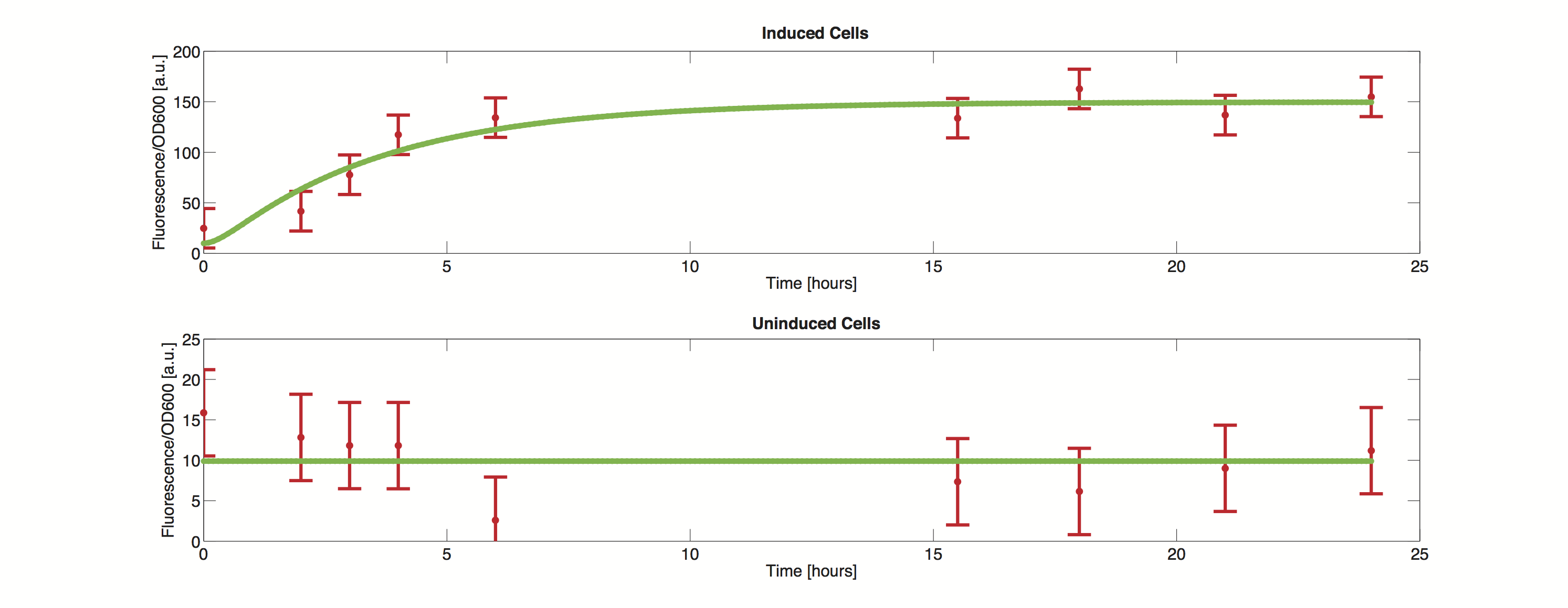
The methods utilized rely on a value for standard deviation, but only one experimental measurement was performed. Hence a value was infered during the optimization process. Thus the error bars in the plot do not reflect values from actual measurements but merely show how well the data can be approximated by the model.
It is clearly visible that the simulated time course stays within the standard deviation and we can thus conclude, that the model is definitely able to reproduce the data.
Profile Likelihood
For the profile likelihood analysis, the scripts provided by the Systems Biology group from TU Eindhovenhttp://bmi.bmt.tue.nl/sysbio/software/pua.html Vanlier and van Riel, 2012 were used and modified to our needs.
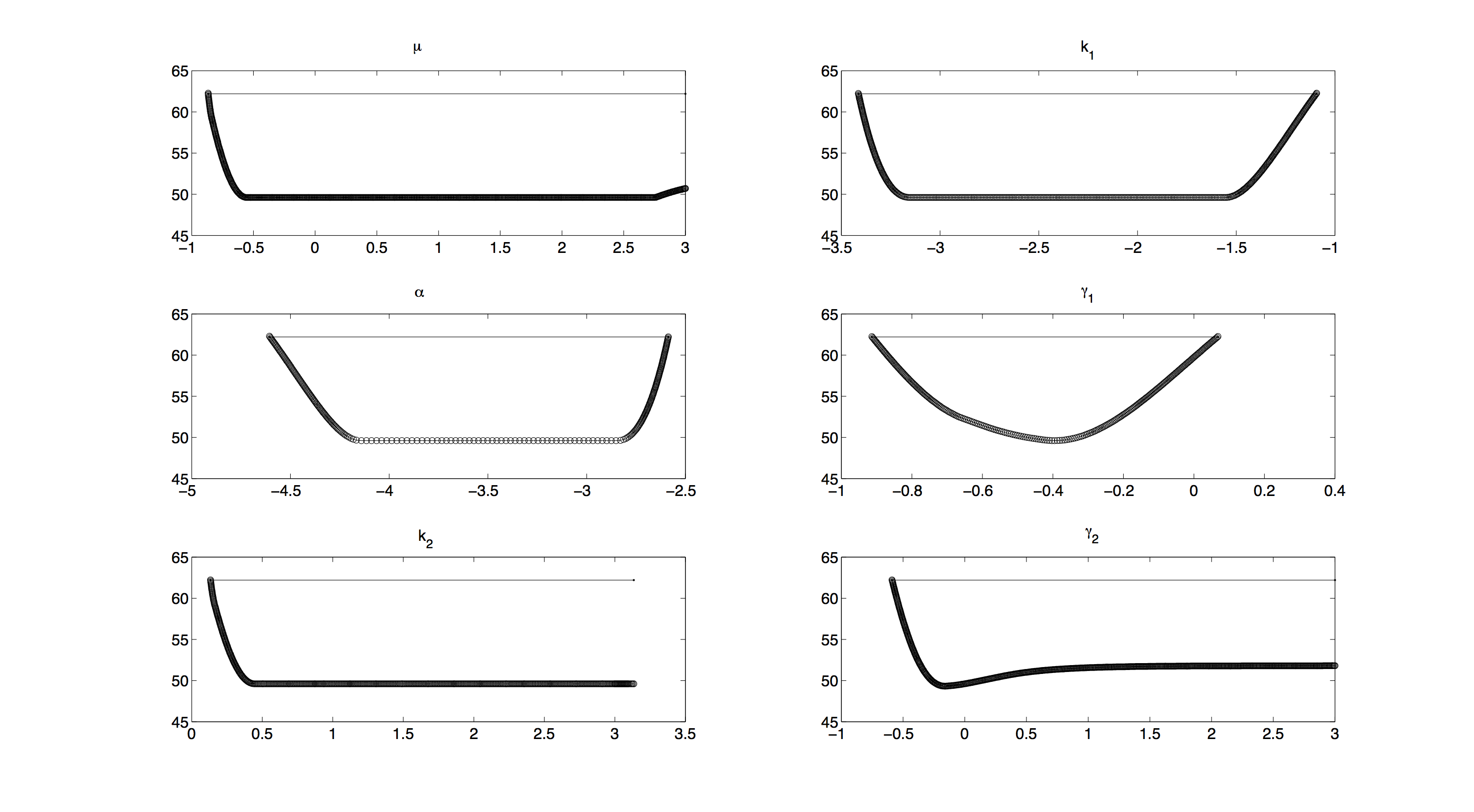
All profiles in figure 2 have a convex shape, which means that we have no structural non-identifiabilitieshttp://www.ncbi.nlm.nih.gov/pubmed/22355081 Vanlier et al., 2012 and all parameters are identifiable. Still all profiles except the one for γ1 have a rather large, flat section in the middle. This means, as long as the prior does not significantly change anything, we will not be able to make very accurate predictions on the parameters.
Including priors in further investigating will increase the accuracy of our measurements. Unfortunately, as computing profile likelihoods can become quite time consuming, we were not able to compute a profile likelihood with priors included.
Markov Analysis
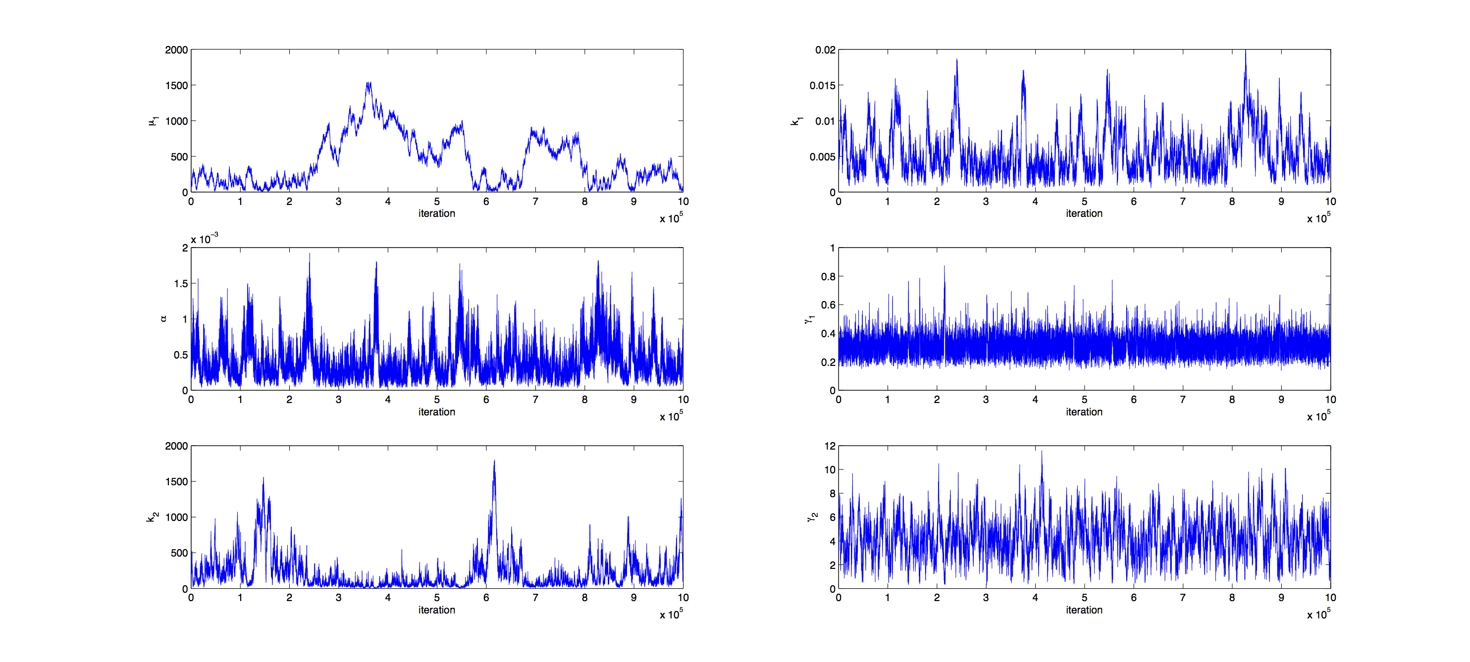
Analysis was performed with a Metropolis Hastings algorithm with a multivariate normal distribution as jumping distribution. 1000000 samples were generated and then thinned by a factor 1:100 to reduce correlation of the samples. The covariance matrix of previously generated samples were used to tune the jumping distribution, this resulted in an acceptance rate of 21%, so a little below the target of 23%.
Joint Distribution
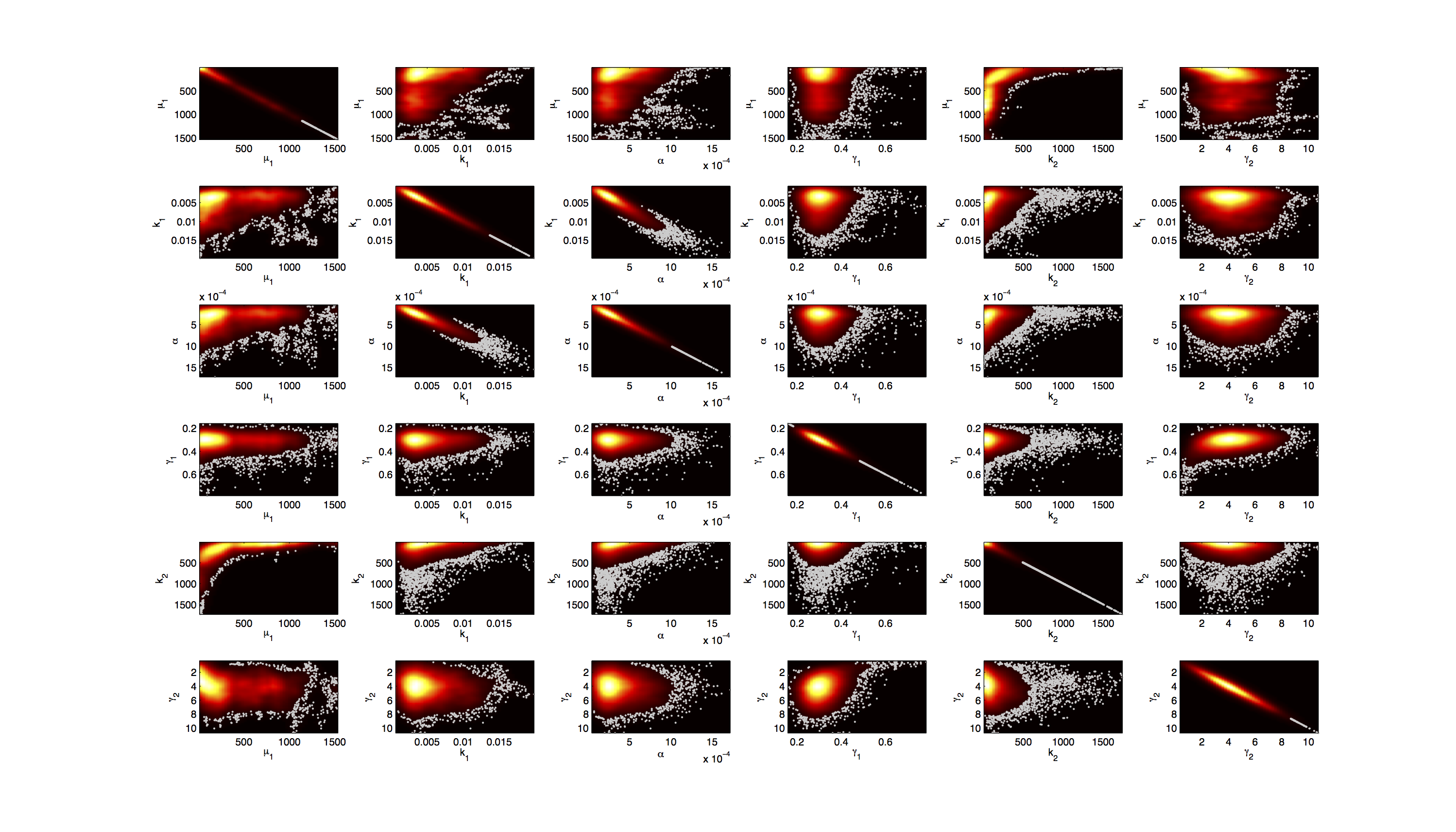
For the smoothed histogram plot smoothhist2d.mhttp://www.mathworks.de/matlabcentral/fileexchange/13352-smoothhist2d Perkins, 2009 was used. The color indicates the density of samples. Black to dark red reflects a low density, yellow to white indicates a high density. Grey dots indicate samples identified as outliers by the script.
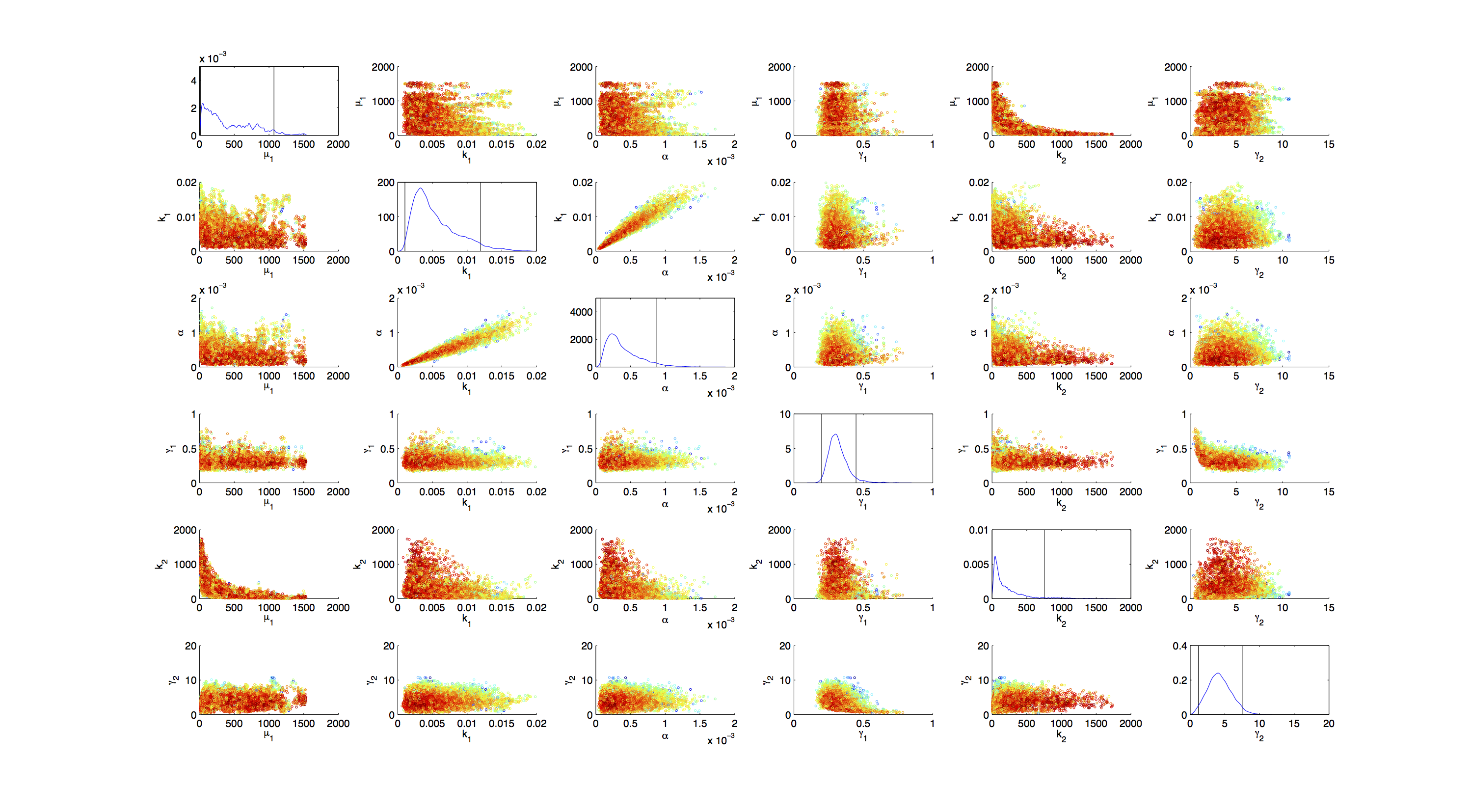
On the diagonal of the scatter plot the kernel density estimation script kde.mhttp://www.mathworks.com/matlabcentral/fileexchange/14034-kernel-density-estimator Botev, 2011 was used to obtain a plot of the respective marginal densities. Off the diagonal is a again a plot of the joint distribution. Here the color indicates the a-posterior probability of the respective sample. Low probabilities are mapped by blue to green color, High probabilities are mapped by yellow to red color.
Mind that due to the nature of the the utilized scripts, the orientation of the Y-Axis is flipped when comparing the two plots.
Credibility Intervals
As the Metropolis Hastings algorithm samples exactly from the target distribution, one can use the generated samples to find credibility intervals. The shown intervals are maximum density credibility intervals. They were obtained by computing the 1-α/2; and α/2 quantiles, with alpha being the missing percentage to 100%, that minimized the 1-norm of the distance between the two values.
| Param. | μ1 | k1 | α | γ1 | k2 | γ2 |
| 95% | [12.382 , 1071.7839] | [0.0010499 , 0.011948] | [6.3391e-05 , 0.00087908] | [0.19995 , 0.44776] | [3.5265 , 752.506] | [1.1874 , 7.5962] |
| 75% | [13.2805 , 689.7555] | [0.0015094 , 0.0075451] | [9.2453e-05 , 0.00053438] | [0.23201 , 0.36719] | [5.7721 , 280.4263] | [2.2895 , 6.204] |
| 50% | [17.3154 , 311.951] | [0.0015555 , 0.0048179] | [0.00012188 , 0.00035519] | [0.25822 , 0.33384] | [16.0541 , 134.1347] | [2.8657 , 5.1221] |
3D plot of resulting timecourse
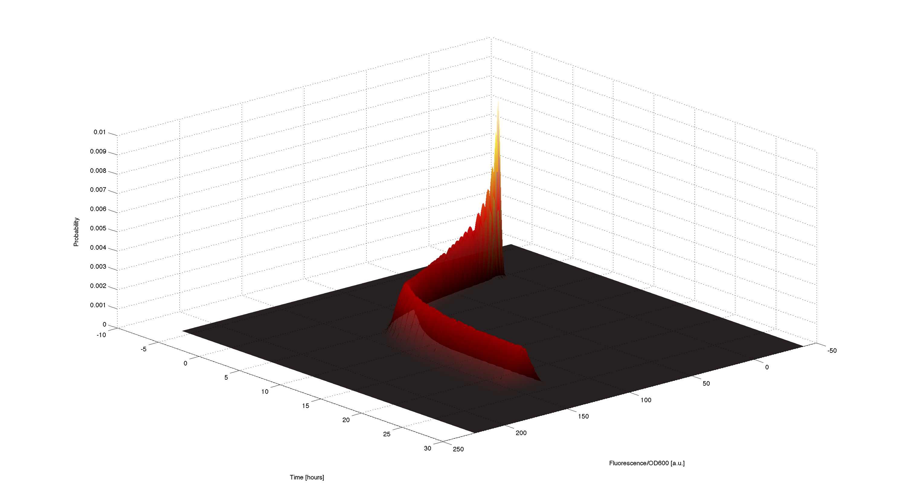
Using the generated samples we can simulate the time course for all of them and use the 2d kernel density estimation script kde2d.mhttp://www.mathworks.com/matlabcentral/fileexchange/17204-kernel-density-estimation Botev, 2009 to plot a distributed time-course of the simulated fluorescence.
Conclusion
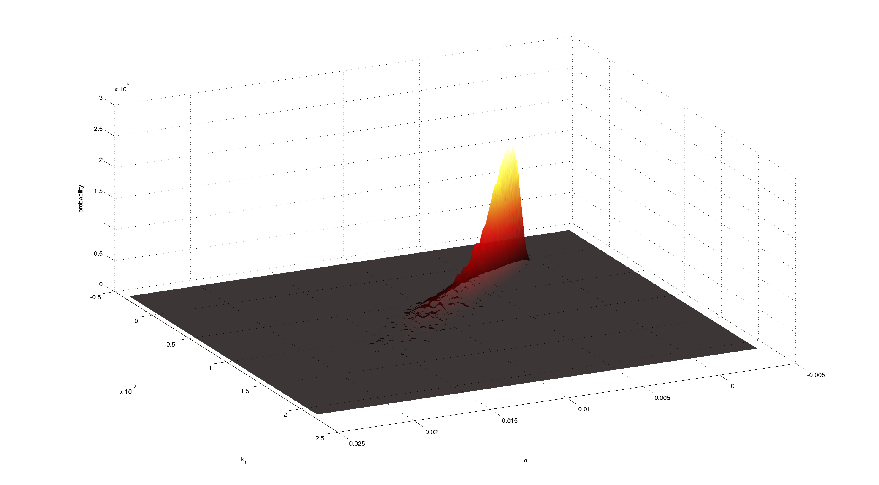
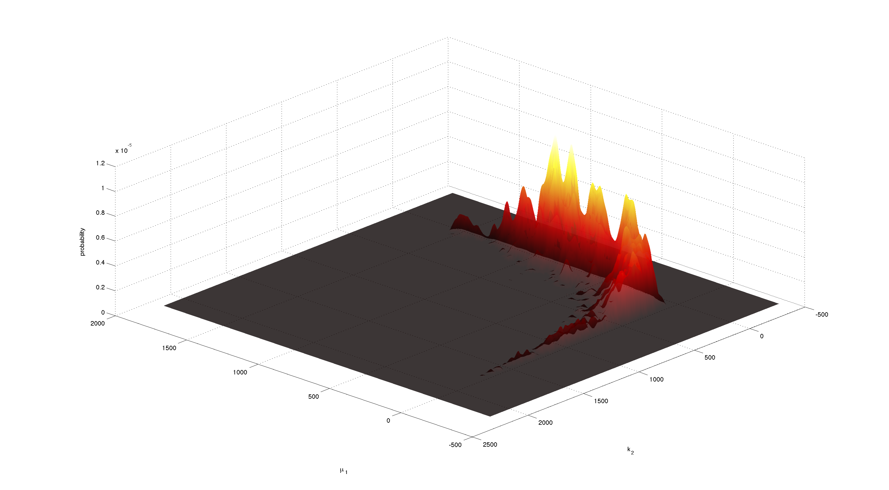
Figures 3-5 all show a strong positive correlation between k1 and α. When looking at figure 7 we see that the joint density of the two parameters has a clear peak. Thus the two parameters should be identifiable.
For parameters μ1 and k2 figure 4 and 5 clearly show a strong negative correlation of the two parameters. The joint distribution in figure 8 suggests no single localized peak, hence those two parameters are most likely non-identifiable.
As the profile likelihood tells us that we should not expect any structural non-identifiabilities, it must be possible to remove this non-identifiability by inclusion of further priors.
This non-identifiability is also reflected in the huge size of the confidence intervals.
Sensitivity Analysis
Differential Equation
Result
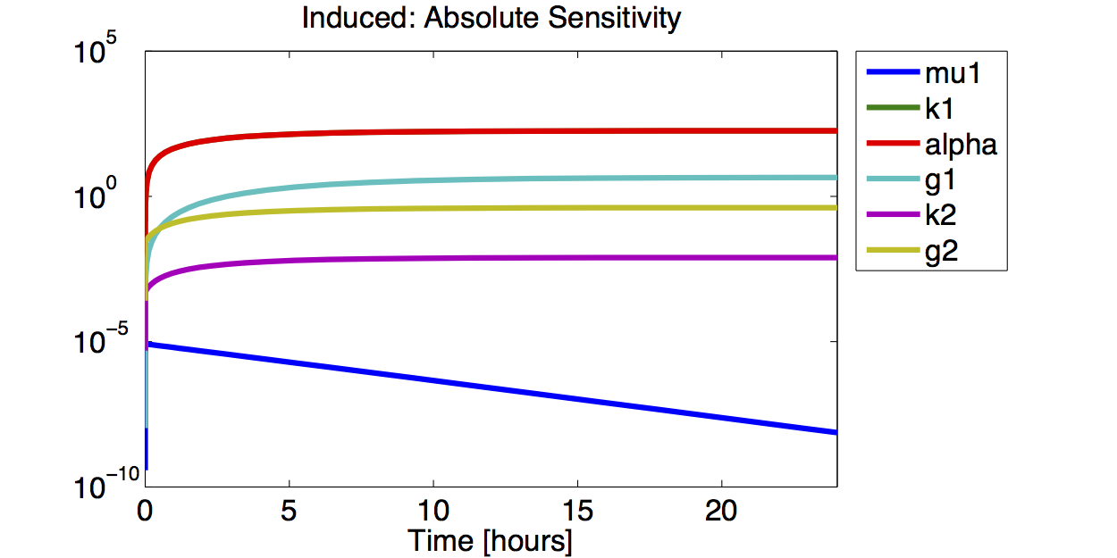
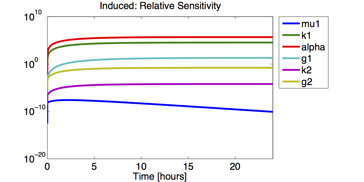
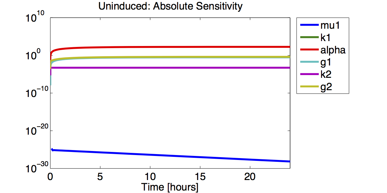
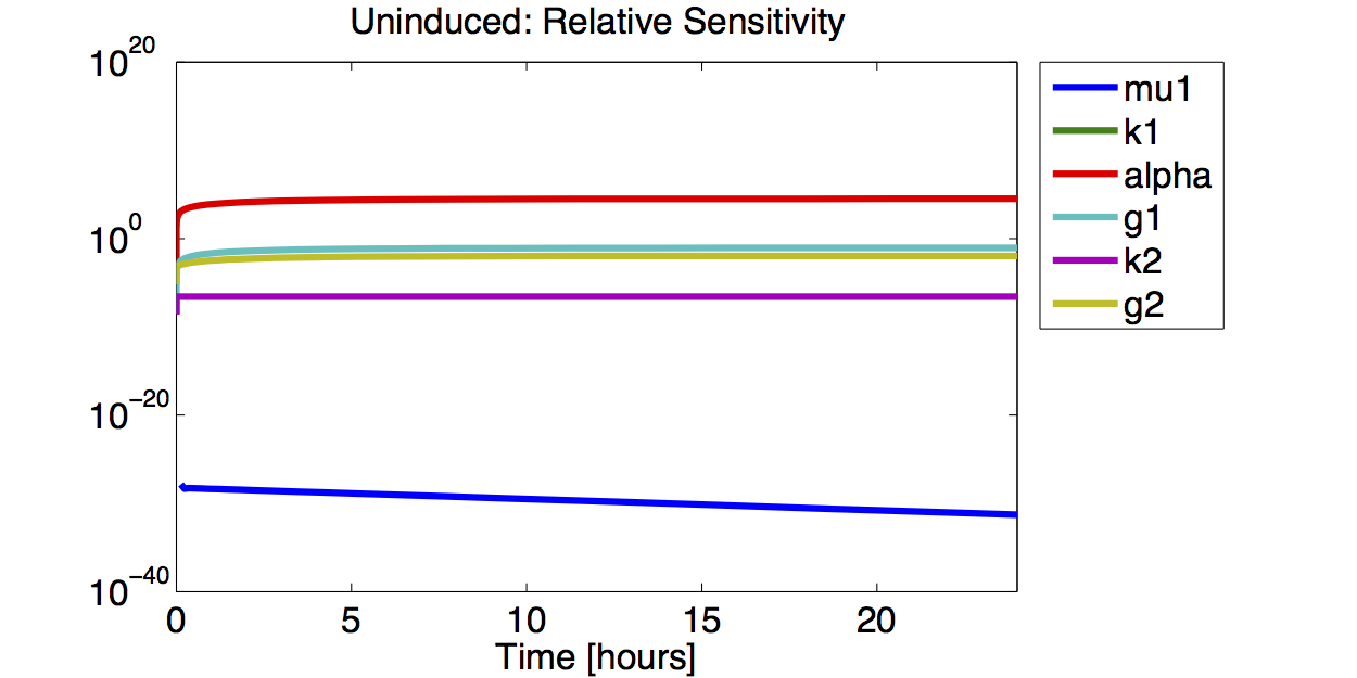
A high sensitivity means that small changes in the parameter will cause large deviations in the resulting simulations. In figure 9 and 10 the magnitude of the curves for the sensitivity of the parameters inversely correlates with the size of the confidence intervals of the respective parameters. This perfectly matches our expectations.
Code
Reference
- http://www.mathworks.com/matlabcentral/fileexchange/17204-kernel-density-estimation Botev, 2009 Botev, Z. (2009). http://www.mathworks.com/matlabcentral/fileexchange/17204-kernel-density-estimation.
- http://www.mathworks.com/matlabcentral/fileexchange/14034-kernel-density-estimator Botev, 2011 Botev, Z. (2011). http://www.mathworks.com/matlabcentral/fileexchange/14034-kernel-density-estimator.
- http://www.mathworks.de/matlabcentral/fileexchange/13352-smoothhist2d Perkins, 2009 Perkins, P. (2009). http://www.mathworks.de/matlabcentral/fileexchange/13352-smoothhist2d.
- http://www.ncbi.nlm.nih.gov/pubmed/22355081 Vanlier et al., 2012 Vanlier, J., Tiemann, C. A., Hilbers, P. A. J., and van Riel, N. A. W. (2012). An integrated strategy for prediction uncertainty analysis. Bioinformatics, 28(8):1130–5.
- http://bmi.bmt.tue.nl/sysbio/software/pua.html Vanlier and van Riel, 2012 Vanlier, J. and van Riel, N. (2012). http://bmi.bmt.tue.nl/sysbio/software/pua.html.
 "
"
