Team:BYUProvo/Modeling
From 2012.igem.org

|

|

|
| Home | Team | Team Profile | Project | Parts | Modeling |
|
Safety | Outreach | Collaboration | Attributions |
Contents |
Introduction
Colon cancer polyps produce high amounts of reactive oxygen species (ROS) and lactate. The high metabolic activity also causes an increase in temperature. Sensors for any one of these inputs alone would be confounded by normal physiological variation in temperature, lactate concentration, and ROS concentration. We propose a genetic circuit designed to detect higher than normal levels of all three, producing two separate outputs. There are two parts to the circuit: The first is a dual input system, using temperature and ROS as inputs to produce an output (LacZ). The second is a single input system, using lactate to produce GFP.
Insert picture of model here
In order to model our system, we have undertaken three main tasks:
1) Create a model using Mass-Action Enzyme Kinematics
2) Analyze this model using computational methods
3) Create an algorithm to predict the structure of our RNA thermosensors
We will start by describing the reactions within our circuit and then by creating a system of differential equations from the reaction sequence.
Our Circuit
Insert picture of circuit here.
The diagram above depicts the inner workings of our circuit created within E. Coli. The following chemical equations depict the pathway:
Insert chemical equations here.
The Model
Mass-Action Equations
Using mass-action kinetics, we write these chemical equations as a system of differential equations.
Insert ODEs here
System of ODEs
As it is, the system is too complicated for us to analyze, so we hereby make a few assumptions to simplify.
- Quasi Steady-State Assumption
- Forward Reaction Assumption
Temperature Dependence
Parameter Estimation
Experimental Data from Lab Work
Analysis
Bifurcation Analysis
Steady State Analysis
Modeling our Thermosensor
Herein we provide detailed information about our library of thermosensors and describe our attempt to model the secondary structure of the RNA hairpins.
Smith-Waterman Algorithm
The Smith-Waterman Algorithm is a simple process used to perform sequence alignment. To demonstrate how the algorithm works, we will use these two sequences:
- ACUAGGUA
- AGCUAGGA
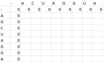
First one sequence is placed in the first row of a grid, skipping the first two entries in the row. The second is likewise placed in the first column, skipping the first two entries in the column. Zeros are then placed in row 2 and column 2.
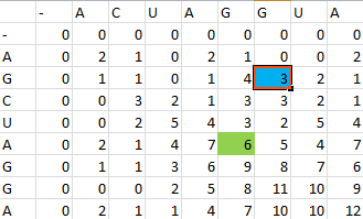
Then, a scoring matrix, S is created according to the following rules:
For example S(4,8) in the blue was obtained by adding 2 to the number in the entry in the upper left-hand corner. S(7,7) was obtained by adding -1 to the max of the 3 numbers above, on the upper left-hand corner, and to the left of it.
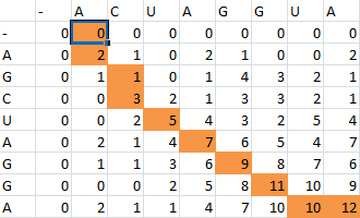
Once the scoring matrix has been completed, starting in the bottom right corner, a path is chosen, picking the largest numbers (only numbers to the left, above or up and to the left can be chosen), until the path arrives back at a zero. When a number above or to the left is the same as the number on the diagonal, the number above or to the left is to be chosen first.
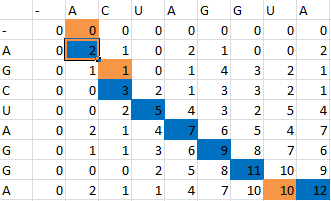
The resulting path spells out the proper alignment of the two sequences. Squares alone in their row and column represent an alignment and when two or more squares share the same column or row, the one closest to the bottom right corner is the one that represents the alignment. The other squares represent deletions or insertions. For our example, the final alignment is shown in the blue.
Thus the alignment of the two sequences would be:
- A--CUAGGUA
- AGCUAGG--A
Our Revised Algorithm
Using the same ideas applied in the Smith-Waterman method, we created an algorithm to model the secondary structure of our RNA thermosensors. The main difference is that we are aligning one side of an RNA sequence with its other side and we are not working with two separate sequences. Thus, we create a similar scoring matrix by placing the RNA sequence along the top row (skipping the first 2 entries) and by placing the reverse of the RNA sequence down the first column (also skipping the first 2 entries).
We then assign priorities in this way:
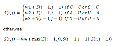
The if statements refer to the alignment of different base pairs. Here, w1, w2, w3 and w4 are weights that we assigned unique to our thermosensors.
- w1 = 1
- w2 = 2
- w3 = 3
- w4 = -2
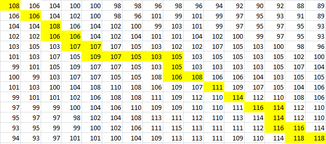
To provide an example, we will use TSA, the wild-type thermosensor. After placing the forward sequence along the top row and the reverse sequence down the first column, we start at the very bottom right corner and proceed to find our way back, following the path that gives us the largest values. The rules for our algorithm are as follows:
- 1) The to go from one entry to another, the largest of the three values in the entries to the left, above and in the left-hand corner is picked.
- 2) If the largest value is present twice, once in the corner and once to the left or above, always choose to move to the left or above before moving to the corner entry and then only move to the corner entry if it is the largest number for the next pick.
- 3) If the largest value is present in both the left entry and the one above(3 times if present in the corner entry as well), choose the one which will largest number in the next pick.
- 4) Continue on this path until the entry S(i,j) has been reached where i+j = n | n = total number of bases in the RNA sequence being analyzed. This represents the point where the thermosensor turns around and you would be, essentially, going back the way you came.
- 5) Then, pick every entry which is connected to another entry only by a corner. Discard all entries which sit in an irregular position. There are 2 types of irregular positions. First, if an entry in the lower right hand corner is less than the entry in the upper left hand corner, discard the entry in the lower right hand corner. Second, if an entry stands alone, not connected to any other entries, discard that entry. See figure above for an example.
Here is the final path:
Here is a breakdown of the color scheme:
- Yellow is the path back determined by our algorithm
- The dark boxes are the entries chosen by our algorithm
- Red are the actual bonding patterns observed in the secondary structure of TSA
- Orange is where the actual bonding patterns fall on the same path predicted by our algorithm
And for a look at the entire S matrix:
 "
"
