Team:Peking/Modeling/Ring/Simulation
From 2012.igem.org
| Line 65: | Line 65: | ||
</table> | </table> | ||
</div> | </div> | ||
| - | + | ||
| - | + | ||
| - | + | ||
| - | + | ||
| - | + | ||
| - | + | ||
| - | + | ||
| - | + | ||
| - | + | ||
| - | + | ||
| - | + | ||
| - | + | ||
| - | + | ||
| - | + | ||
| - | + | ||
| - | + | ||
| - | + | ||
| - | + | ||
| - | + | ||
| - | + | ||
<p> | <p> | ||
The simulation result is shown below: | The simulation result is shown below: | ||
| Line 92: | Line 74: | ||
<div> | <div> | ||
<p class="description" style="text-align:center;"> | <p class="description" style="text-align:center;"> | ||
| - | Figure 1. ODE Simulation Result of the | + | Figure 1. ODE Simulation in a plate of the ring-like pattern formation. |
| + | </p> | ||
| + | </div> | ||
| + | <img src="/wiki/images/b/bd/Band_Origin_2.png" alt="Simulation Result" style="width:600px;"/> | ||
| + | <div> | ||
| + | <p class="description" style="text-align:center;"> | ||
| + | Figure 2. ODE Simulation for the radial expression amplitude of the ring-like pattern formation. | ||
</p> | </p> | ||
</div> | </div> | ||
| Line 101: | Line 89: | ||
</div> | </div> | ||
<div class="PKU_context floatR"> | <div class="PKU_context floatR"> | ||
| - | <h3 id="title2"> | + | <h3 id="title2">Parameter Analysis</h3> |
<p> | <p> | ||
In order to verify the robustness of <i>Luminesensor</i> function, we simulated this reaction network with a <!--<a href="/Team:Peking/Modeling/Appendix/Stochastic">-->stochastic model<!--</a>-->. By estimating the volume of a cell, we converted the concentration of a component into the number of molecules by 1 n mol/L : 1. The results are shown below: | In order to verify the robustness of <i>Luminesensor</i> function, we simulated this reaction network with a <!--<a href="/Team:Peking/Modeling/Appendix/Stochastic">-->stochastic model<!--</a>-->. By estimating the volume of a cell, we converted the concentration of a component into the number of molecules by 1 n mol/L : 1. The results are shown below: | ||
Revision as of 02:46, 23 October 2012
ODE Model
According to the previous circuit and ODE model, we listed all the differential equations and simulated this system with MATLAB with equations listed as below:
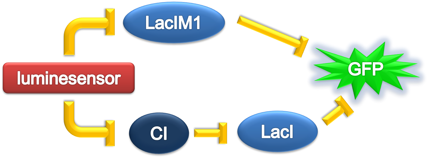
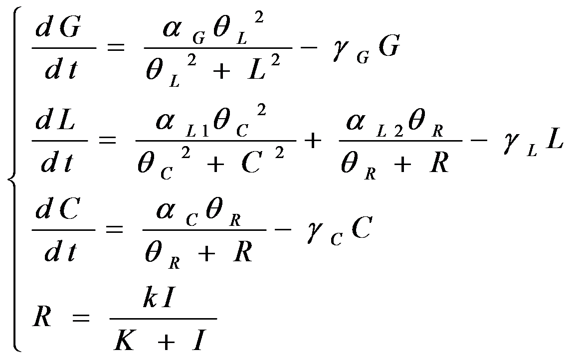
And parameters as
| Parameter | Value | Unit | Description | Source |
| k1 | 3.x10-4 | s-1 | vivid decay rate constant | |
| k2 | 5.6x10⁻⁵ | s-1 | vivid dissociation rate constant | [3] |
| k3 | 8.x10-4 | s-1 | monomer LexA releasing rate constant from specific binding site | |
| k4 | 1.x10-3 | s-1 | binded monomer LexA dissociation rate constant | |
| k5 | 1.x10-4 | s-1 | dimered LexA releasing rate constant from specific binding site | |
| K1(Dark) | 0 | 1 | equilibrium excitation constant on dark | |
| K1(Light) | 1.x10+3 | 1 | equilibrium excitation constant on light | |
| K2 | 7.7x10⁻⁵ | (n mol/L)-1 | vivid association equilibrium constant | [1] |
| K3 | 1.x10-3 | (n mol/L)-1 | monomer LexA binding equilibrium constant with specific binding site | [2] |
| K4 | K2xK5/K3 | (n mol/L)-1 | binded monomer LexA association equilibrium constant | Thermal Principle |
| K5 | 1. | (n mol/L)-1 | dimered LexA binding equilibrium constant | [2] |
| [LG]0 | 1000 | n mol/L | initial concentration of Luminesensor in ground state | |
| [LA]0 | 0 | n mol/L | initial concentration of Luminesensor in active state | |
| [LA2]0 | 0 | n mol/L | initial concentration of dimered Luminesensor | |
| [DL]0 | 100 | n mol/L | initial concentration of free specific binding site on DNA | high-copy plasmid |
| [LGDL]0 | 0 | n mol/L | initial concentration of dimered Luminesensor binded Luminesensor in ground state | |
| [LADL]0 | 0 | n mol/L | initial concentration of dimered Luminesensor binded Luminesensor in active state | |
| [LA2DL]0 | 0 | n mol/L | initial concentration of binded and dimered Luminesensor |
The simulation result is shown below:
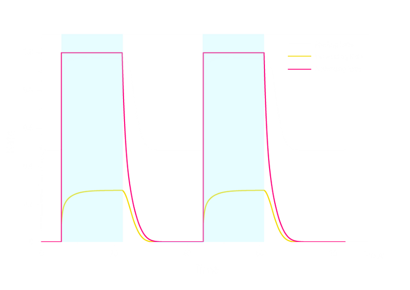
Figure 1. ODE Simulation in a plate of the ring-like pattern formation.

Figure 2. ODE Simulation for the radial expression amplitude of the ring-like pattern formation.
From the Figure 1 above, we discovered that the activation and decay of Luminesensor are the key points of progress, and the activating rate is the most sensitive to light intensity. The promoter will be repressed even though the Luminesensor does not totally dimerized.
Parameter Analysis
In order to verify the robustness of Luminesensor function, we simulated this reaction network with a stochastic model. By estimating the volume of a cell, we converted the concentration of a component into the number of molecules by 1 n mol/L : 1. The results are shown below:
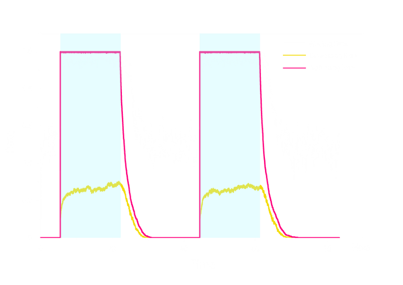
Figure 2. Stochastic Simulation Result of Prototype Luminesensor.
According to Figure 2 above, noise does not influence this system. Thus the Luminesensor is expected to work theoretically. Besides, the average value of stochastic simulation is consistent with the result of ODE model, which in turn proves the self-consistency of our ODE model.
Simulation for GFP Expression
Regulated by the Luminesensor
In order to see whether our model is predictive for the downstream gene expression under control of the Luminesensor, transcription and translation process were incorporated into the modeling of DNA binding process. In addition, we considered the delay of translation initiation time and the growth of cell. The simulation below(Figure 3) represents the GFP expression regulated by the Luminesensor. After a long time in light condition, where GFP expression is inhibited, from t=0h, the cells are moved into dark and begin to express GFP. The GFP expression level varying with time was recorded in this simulation.
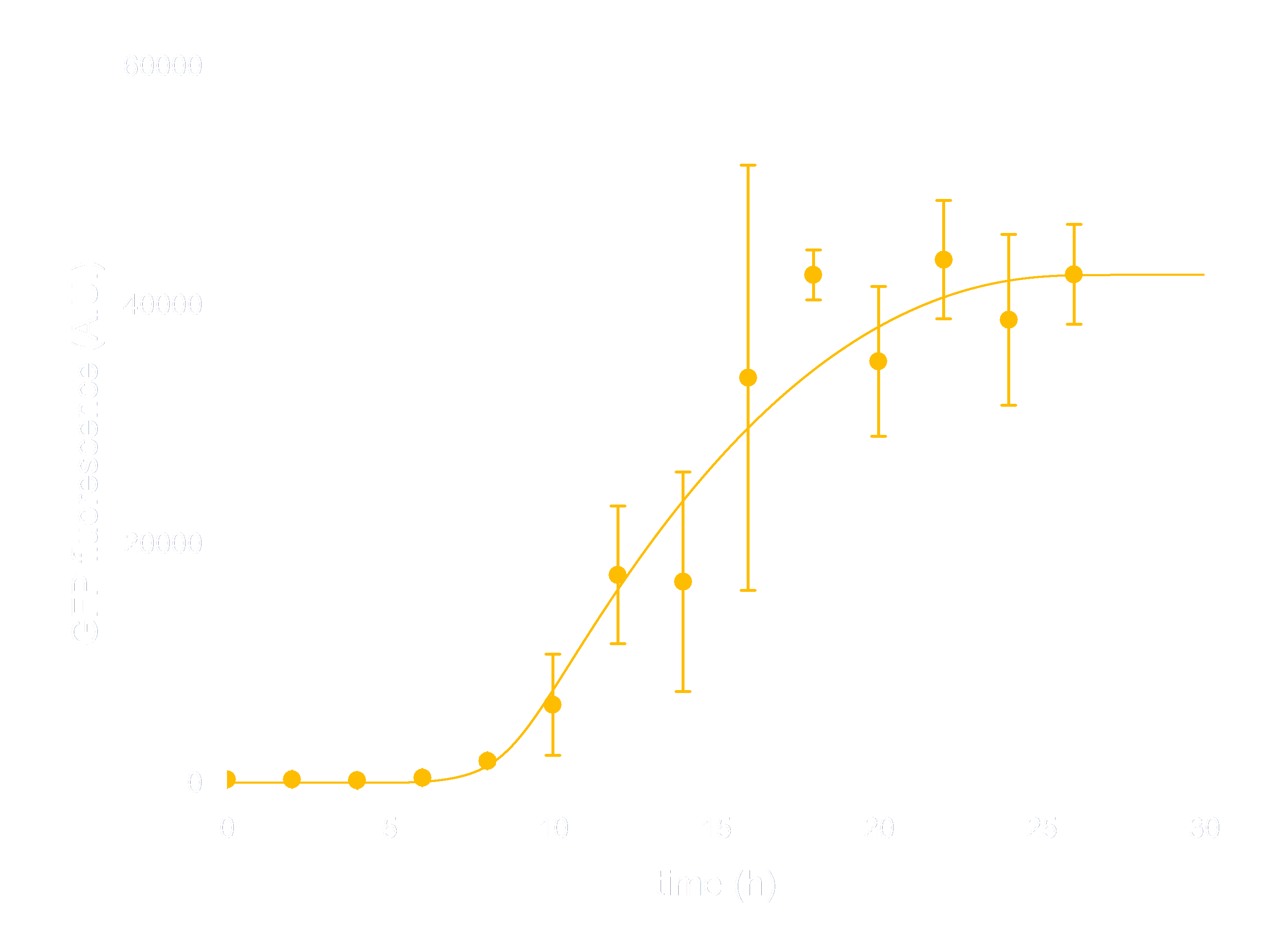
Figure 3. ODE Simulation Result is correspond to the experiment data of GFP expression level according to time from, which suggests that our model is effective to present the experiment situation.
Reference
- 1. Zoltowski, B.D., Crane, B.R.(2008). Light Activation of the LOV Protein Vivid Generates a Rapidly Exchanging Dimer. Biochemistry, 47: 7012: 7019
- 2. Mohana-Borges, R., Pacheco, A.B., Sousa, F.J., Foguel, D., Almeida, D.F., and Silva, J.L. (2000). LexA repressor forms stable dimers in solution. The role of specific DNA in tightening protein-protein interactions. J. Biol. Chem., 275: 4708: 4712
- 3. Zoltowski, B.D., Vaccaro, B., and Crane, B.R. (2009). Mechanism-based tuning of a LOV domain photoreceptor. Nat. Chem. Biol. 5: 827: 834
 "
"


