Team:TU Munich/Modeling/Priors
From 2012.igem.org
| Line 7: | Line 7: | ||
<div class="show"> | <div class="show"> | ||
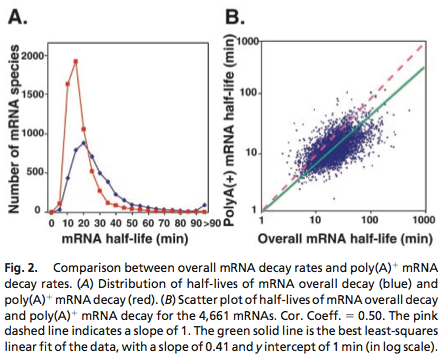
[[File:TUM12_mRNA_degradation.png|300px|thumb|right|'''Fig. 1''' Genome-wide mRNA decay rate. Picture taken from Wang et. al. 2002]] | [[File:TUM12_mRNA_degradation.png|300px|thumb|right|'''Fig. 1''' Genome-wide mRNA decay rate. Picture taken from Wang et. al. 2002]] | ||
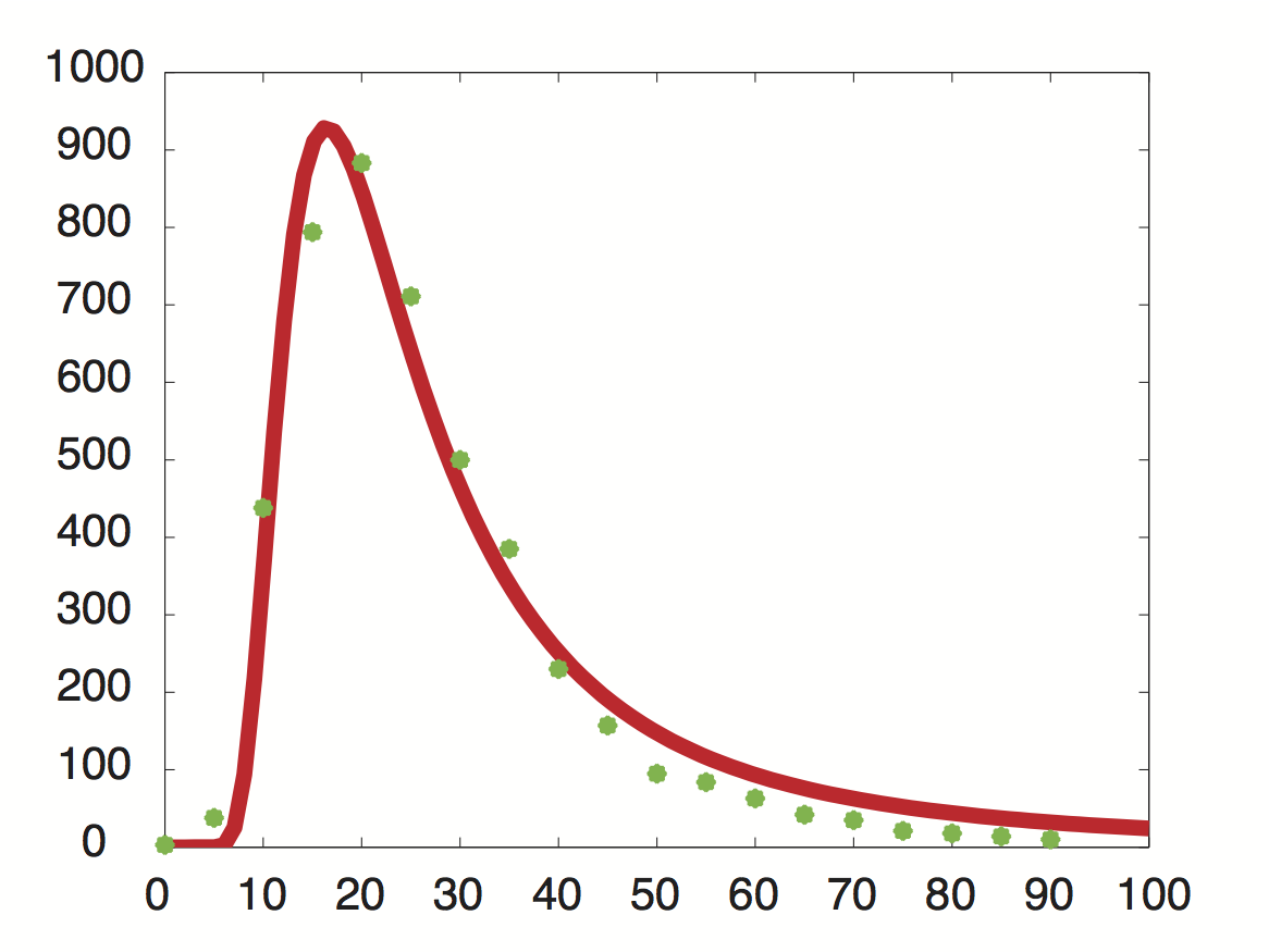
| - | [[File:TUM12_PriormRNAdecay.jpg| | + | [[File:TUM12_PriormRNAdecay.jpg|300px|thumb|right|'''Fig. 2''' Approximated probability density for the genome-wide mRNA decay rate.]] |
Data was obtained from the Paper [[http://www.ncbi.nlm.nih.gov/pubmed/11972065 Wang et al., 2002]] and processed by [[http://arohatgi.info/webplotdigitizer/app/ Rohatgi, 2012]] to obtain raw data. | Data was obtained from the Paper [[http://www.ncbi.nlm.nih.gov/pubmed/11972065 Wang et al., 2002]] and processed by [[http://arohatgi.info/webplotdigitizer/app/ Rohatgi, 2012]] to obtain raw data. | ||
Using a least-squared error approximation the distribution of the half life time in was approximated as '''noncentral ''t''-distribution''' with parameters μ = 1.769 and ν = 20.59. | Using a least-squared error approximation the distribution of the half life time in was approximated as '''noncentral ''t''-distribution''' with parameters μ = 1.769 and ν = 20.59. | ||
| Line 78: | Line 78: | ||
<div> | <div> | ||
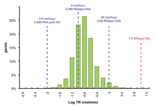
[[File:TUM12_mRNA_transcription.png|300px|thumb|right|'''Fig. 3''' Genome-wide transcription rate. Picture taken from Pelechano et al. 2010]] | [[File:TUM12_mRNA_transcription.png|300px|thumb|right|'''Fig. 3''' Genome-wide transcription rate. Picture taken from Pelechano et al. 2010]] | ||
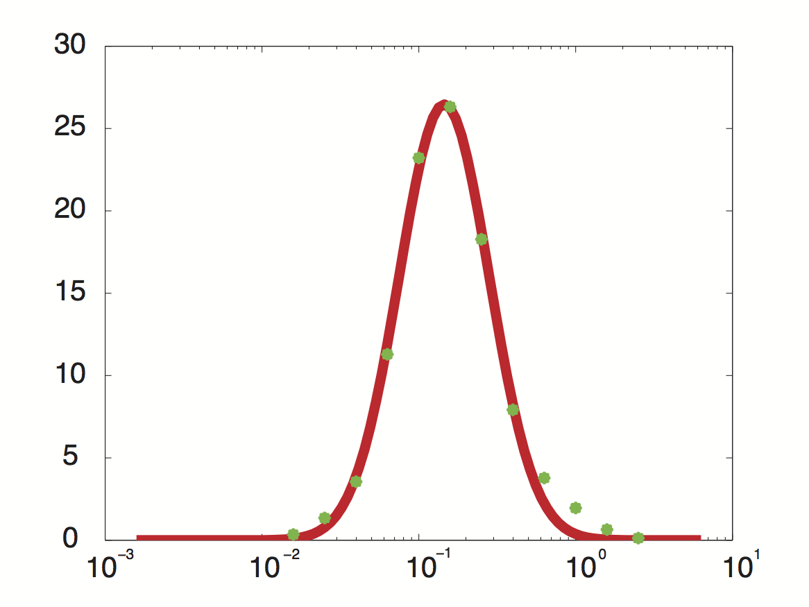
| - | [[File:TUM12_PriormRNAtrans.jpg| | + | [[File:TUM12_PriormRNAtrans.jpg|300px|thumb|right|'''Fig. 4''' Approximated probability density for the genome-wide transcription rate.]] |
Data was obtained from the Paper [[http://www.ncbi.nlm.nih.gov/pubmed/21103382 Pelechano et al., 2010]] and processed by [[http://arohatgi.info/webplotdigitizer/app/ Rohatgi, 2012]] to obtain raw data. | Data was obtained from the Paper [[http://www.ncbi.nlm.nih.gov/pubmed/21103382 Pelechano et al., 2010]] and processed by [[http://arohatgi.info/webplotdigitizer/app/ Rohatgi, 2012]] to obtain raw data. | ||
Using a least-squared error approximation the distribution of the transcription rate was approximated as '''log-normal distribution''' with parameters μ = -1.492 and σ = 0.661;. | Using a least-squared error approximation the distribution of the transcription rate was approximated as '''log-normal distribution''' with parameters μ = -1.492 and σ = 0.661;. | ||
Latest revision as of 19:43, 26 October 2012


Contents |
Prior Data
Yeast mRNA Degradation Rate
Data was obtained from the Paper http://www.ncbi.nlm.nih.gov/pubmed/11972065 Wang et al., 2002 and processed by http://arohatgi.info/webplotdigitizer/app/ Rohatgi, 2012 to obtain raw data. Using a least-squared error approximation the distribution of the half life time in was approximated as noncentral t-distribution with parameters μ = 1.769 and ν = 20.59.
dataGraph = [
0.0018691649126431735,0.0016851538590669062
0.05978099456360327,0.01885629059542104
0.11548146330755026,0.21910551258377348
0.17122389948476902,0.396902157771723
0.2253457470848775,0.4417136917136917
0.2815821076690642,0.3552607791738227
0.3359848142456839,0.249812760682326
0.39216629434020744,0.19272091011221448
0.4465173486912618,0.11490683229813668
0.5026600896166115,0.07854043723608946
0.5569239808370243,0.04735863431515607
0.6111394480959699,0.04208365077930302
0.667233765059852,0.031624075102336016
0.7233280820237343,0.021164499425369035
0.777540321018582,0.017616637181854626
0.8373665112795547,0.010604847561369285
0.8897063570976615,0.008787334874291503
0.9420462029157682,0.006969822187213598
0.9999935434718044,0.005142624707842157
];
%scale the data
X = round(dataGraph(:,1)*90);
y = round(dataGraph(:,2)*2000);

k(1) = 1.769292045467269;
k(2) = 20.589996419308118;
k(3) = 24852.48237036381;

k=fminunc(@(z) sum((y-z(3)*nctpdf(X,z(1),z(2))).^2),k);
k=fminunc(@(z) sum((y-z(3)*nctpdf(X,z(1),z(2))).^2),k);
k=fminunc(@(z) sum((y-z(3)*nctpdf(X,z(1),z(2))).^2),k);
k=fminunc(@(z) sum((y-z(3)*nctpdf(X,z(1),z(2))).^2),k);
k=fminunc(@(z) sum((y-z(3)*nctpdf(X,z(1),z(2))).^2),k);
The matlab nctpdf.m script needs to compute the limit of an infinite series to calculate the probabilities for the noncentral t-distribution. As this the function will be called several million times during the generation of samples, the computation was quite time consuming and the funtion was approximated using chebyshev interpolation http://www2.maths.ox.ac.uk/chebfun/ Trefethen, 2012.
Yeast Protein Degradation Rate
For the Degradation Rate the N-end rule http://www.ncbi.nlm.nih.gov/pubmed/9112437 Varshavsky, 1997 served as approximation for the half life time. It states that the half life time in S. cerevisiae can be approximated based on the amino acid after the initial start codon.
| Residue ! Half-life | |
|---|---|
| Arg | 2 min |
| Lys, Phe, Leu, Trp, His, Asp, Asn | 3 min |
| Tyr, Gln | 10 min |
| Ile, Glu | 30 min |
| Pro | > 5 h |
| Cys, Ala, Ser, Thr, Gly, Val, Met | > 30 h |
As these values do not give enough information to infer a proper distribution, only the two lower bounds 5 h and 30 h will serve as approximate lower bounds for the optimization routines.
Yeast Transcription Rate
Data was obtained from the Paper http://www.ncbi.nlm.nih.gov/pubmed/21103382 Pelechano et al., 2010 and processed by http://arohatgi.info/webplotdigitizer/app/ Rohatgi, 2012 to obtain raw data. Using a least-squared error approximation the distribution of the transcription rate was approximated as log-normal distribution with parameters μ = -1.492 and σ = 0.661;.
dataGraph = [
-1.8,0.3442950751957339
-1.6,1.3525375039897853
-1.4,3.5492668181220783
-1.2,11.28874786429094
-1.0,23.213749272450762
-0.8,26.31522126884587
-0.6,18.273455248681024
-0.4,7.913623476840467
-0.2,3.7755111620134825
0,1.9559339854677913
0.2,0.6458759692833385
0.4,0.12767315671880167
];

x = 10.^dataGraph(:,1);
y = dataGraph(:,2);

k(1) = -0.8;
k(2) = 0.2;
k(3) = 25;

k=fminunc(@(z) sum((y-z(3)*lognpdf(x,z(1),z(2))).^2),k);
k=fminunc(@(z) sum((y-z(3)*lognpdf(x,z(1),z(2))).^2),k);
k=fminunc(@(z) sum((y-z(3)*lognpdf(x,z(1),z(2))).^2),k);
k=fminunc(@(z) sum((y-z(3)*lognpdf(x,z(1),z(2))).^2),k);
Reference
- http://www.ncbi.nlm.nih.gov/pubmed/21103382 Pelechano et al., 2010 Pelechano, V., Chávez, S., and Pérez-Ortín, J. E. (2010). A complete set of nascent transcription rates for yeast genes. PLoS One, 5(11):e15442.
- http://arohatgi.info/webplotdigitizer/app/ Rohatgi, 2012 Rohatgi, A. (2012). http://arohatgi.info/webplotdigitizer/app/.
- http://www2.maths.ox.ac.uk/chebfun/ Trefethen, 2012 Trefethen, N. (2012). http://www2.maths.ox.ac.uk/chebfun/.
- http://www.ncbi.nlm.nih.gov/pubmed/9112437 Varshavsky, 1997 Varshavsky, A. (1997). The n-end rule pathway of protein degradation. Genes Cells, 2(1):13–28.
- http://www.ncbi.nlm.nih.gov/pubmed/11972065 Wang et al., 2002 Wang, Y., Liu, C. L., Storey, J. D., Tibshirani, R. J., Herschlag, D., and Brown, P. O. (2002). Precision and functional specificity in mrna decay. Proc Natl Acad Sci U S A, 99(9):5860–5.
 "
"


