Team:Cambridge/Project/Results
From 2012.igem.org


Contents |
Results
Set out below are the developments the team has made over the summer, in tackling our aim and objectives.
RiboSense
Having obtained our DNA, the first test was a rather crude β-Galactosidase assay, the results of which are shown below, the protocol for which is found here.
These results were very positive as it hinted at a good correlation between fluoride concentration and reporter output.
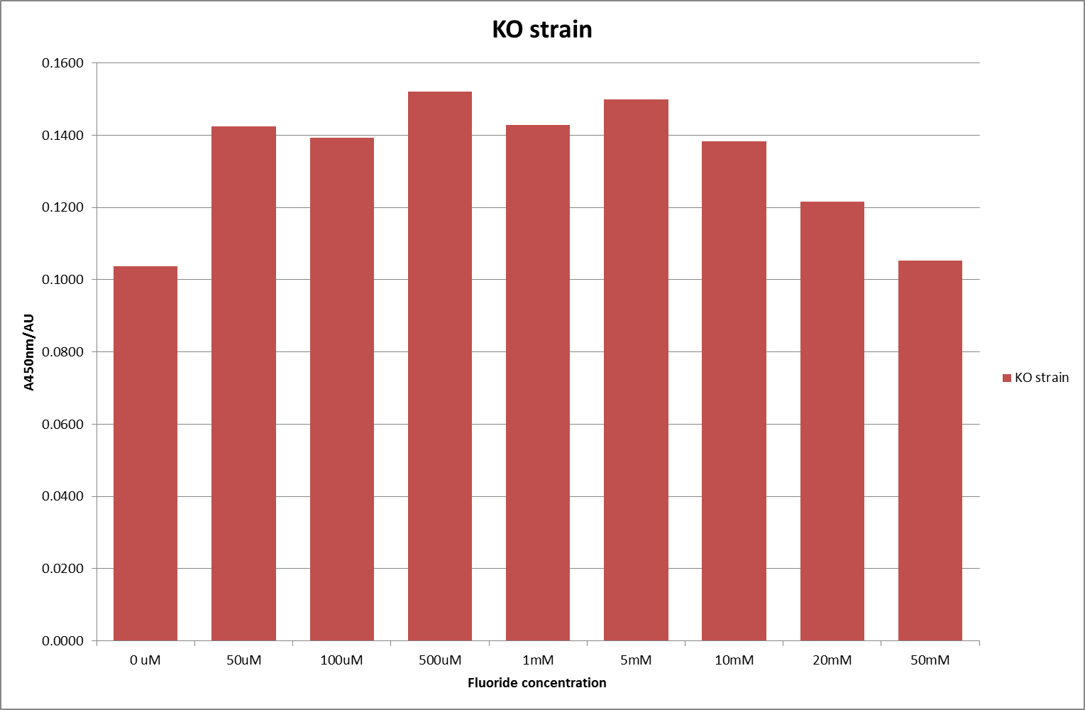
The next step was a more quantitave assay using a 96 well plate reader. This was in line with the assays done in the original paper by Breaker et al. In the paper they carried out a Miller assay, and whilst we have included the full and correct protocol on our protocols page, including the appropriate calculations, we lacked the filters and so were only able to record the A450nm. We feel that this was close enough in wavelength to be a suitable proxy for the A420nm reading required to assay the o-nitrophenol produced. We ran an initial assay and indicative results are below. All the A450 bar charts are based on two repeats, error bars are not included as they would not be statistically significant.
This data seems to show a trend, that at low fluoride concentrations there is a positive relationship between concentration and A450, the A 450 then plateaus, and then at high fluoride concentration the A450 drops again. A possible explanation for this is that there are two conflicting effects, an increase in fluoride leads to an increase in β-galactosidase expression which, in turn, leads to an increased A450. However, the increased fluoride concentrations begin to become toxic and so limit the cell’s ability to produce β-galactosidase, leading to a reduction in A450. It would also seem that the linear region of the initial positive relationship seems to lie between 0μM and 100μM. We therefore repeated the assay, with a longer time course, and with greater resolution in this range, in order to see if the original trend could be reproduced, and also to better quantify this initial correlation. Included below are the results for the repeated assay.
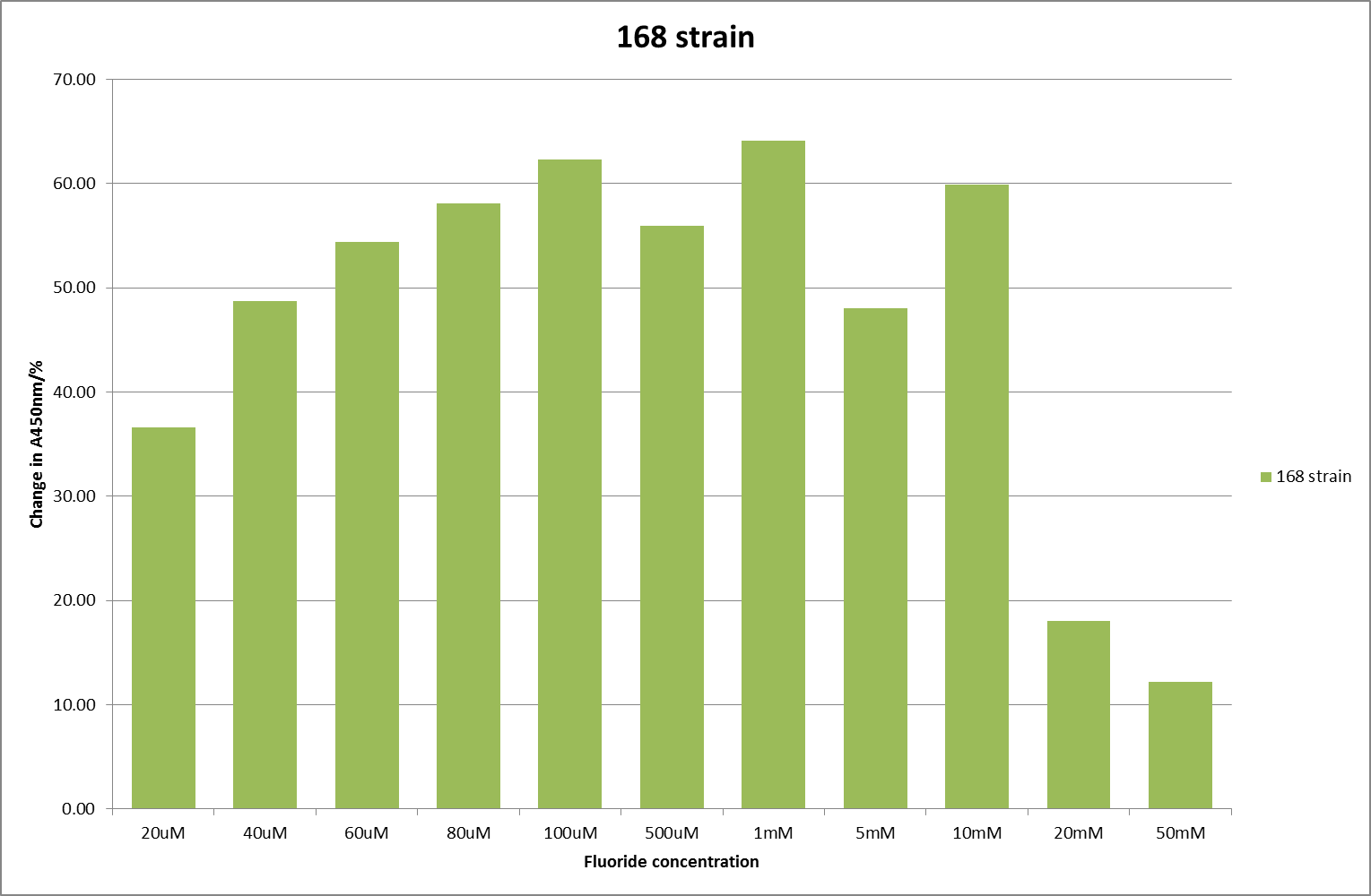
For clarity, and to act as an internal control, the bar chart results are expressed as a percentage change from the same culture, after the same length of time, but with no fluoride added. This data seems to confirm the initial findings, as well as giving greater resolution in the 0μM to 100μM range. The results for higher fluoride concentrations do not seem to quite fit the trend, but as this is consistent across all the cell types it is possible that this was due to errors in making up the solutions, rather than actually being representative of the riboswitch. This data is very encouraging as the WHO safe limit for fluoride is 1.5mg/L (according to [http://dx.doi.org/10.1016/j.envpol.2006.05.007Farooqi et al] ) which works out at 79μM. This means our riboswitch is at its most accurate around the safe level for humans. For more information on the implications of this, have a look at our human practices page .
It should be noted that we expected a greater difference in sensitivity between the knockout Bacillus strain provided by Yale, the 168 strain we were using, and the E. coli we used. In the original paper there was a significant, nearly 100-fold, difference in sensitivity between the knock and wild type bacillus strains, but our data did not reproduce this. However, we feel it is actually very positive as it means our part is consistent across multiple chasses, and that it has the desired sensitivity to fluoride, without the need for a special mutant to be ordered. This fits with our goal for our kit to be a standard which is widely compatible.
The next step was to place this construct in a ratiometric fluorescent construct, before eventually testing our luciferase construct with it. But, due to delays in developing the ratiometric construct, we only had one attempt at inserting and testing it and it proved unsuccessful. We shall carry on testing it and, whilst we cannot put our results on here due to the wiki freeze, we hope to present them to you at the jamborees. However, we would like to include here what we plan to do, in order that future teams might benefit. We plan to insert the fluoride riboswitch into the ratiometrica construct and check that they work together as expected, i.e. get consistent readings for various concentrations, in spite of varying cell densities.
Ratiometrica
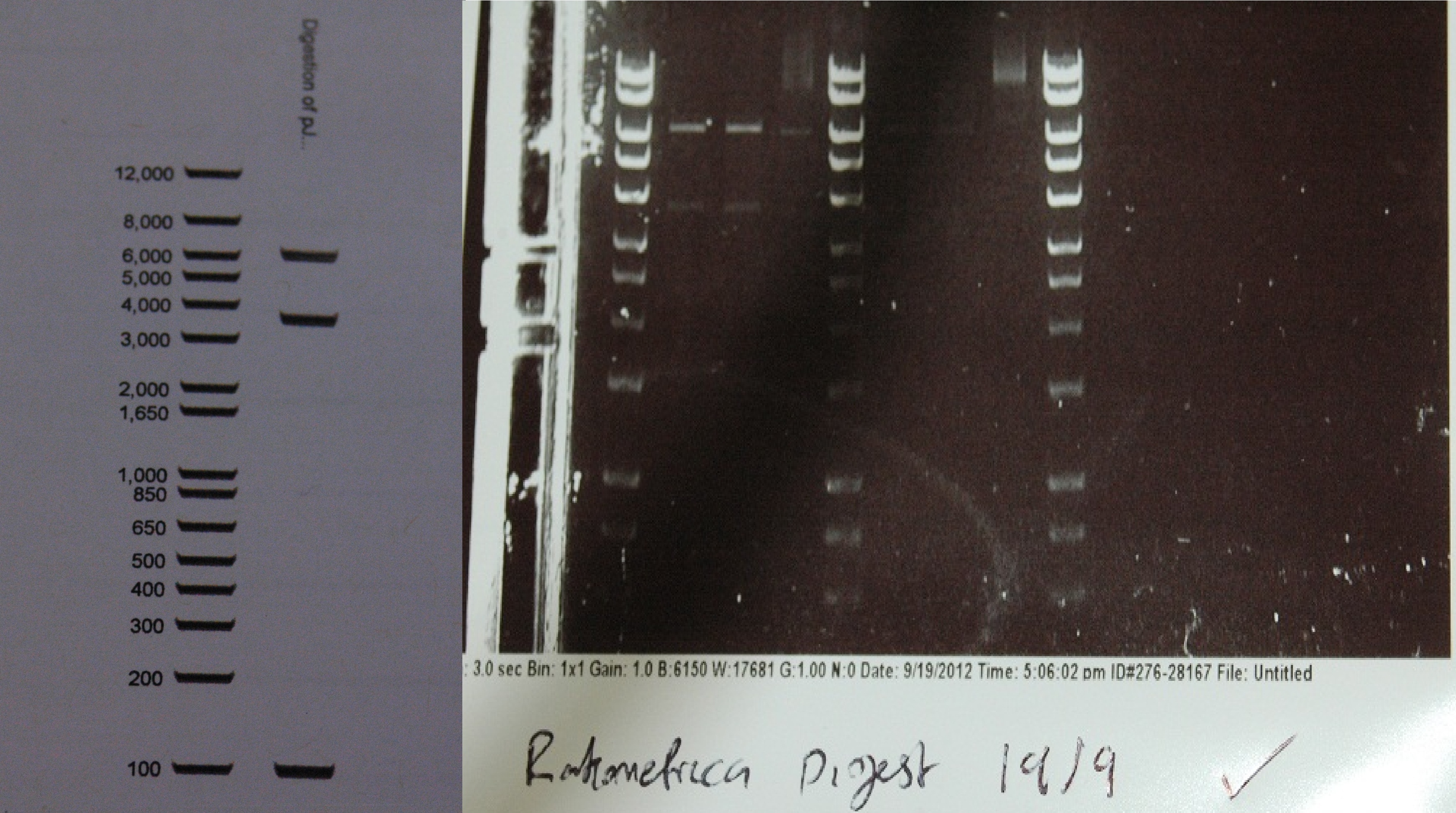
After a lot of technical difficulties, we were able to assemble our fluorescent construct using Gibson assembly. The photo below shows the predicted and obtained digest pattern using HINDIII.
The construct is also sequenced from the beginning and middle (as it is a long part) by Source Bioscience, below is the alignment data from the sequencing (using ClustalW2):
CLUSTAL 2.1 multiple sequence alignment


seq                            ---------------------------NNNNNNNNNNNAANNNNNNNA-- 21
pJS150_seq_-_Ratiometrica      AGCCCAGTCCAGACTATTCGGCACTGAAATTATGGGTGAAGTGGTCAAGA 1050
                                                            .. ......**.....  *

seq                            ---------------------------------------NNNNNNNTNTN 32
pJS150_seq_-_Ratiometrica      CCTCACTAGGCACCTTAAAAATAGCGCACCCTGAAGAAGATTTATTTGAG 1100
                                                                       ... ..*.:.

seq                            GTN--CNNT----------------------------------------- 39
pJS150_seq_-_Ratiometrica      GTAGCCCTTGCCTACCTAGCTTCCAAGAAAGATATCCTAACAGCACAAGA 1150
                               **   * .*

seq                            -----------TTNNNNTCTN-------------CTAANTNTNAGNGCTC 65
pJS150_seq_-_Ratiometrica      GCGGAAAGATGTTTTGTTCTACATCCAGAACAACCTAATTGTGAGCGCTC 1200
                                          **....***              ****.*.*.** ****

seq                            NNAATTTTTTGNNNAATTNNTNANNNTTTATCTACN-GGTGTGTCAT-AT 113
pJS150_seq_-_Ratiometrica      ACAATTTTTTGCAAAAAGTTGTTGACTTTATCTACAAGGTGTGGCATAAT 1250
                                 *********   **: .. .:.  *********  ****** *** **

seq                            GTNTGGAANNNCNANNAGCTCACAATTAANGGATGAATTCN-AATGGTGA 162
pJS150_seq_-_Ratiometrica      GTGTGGAATTGTGAGCGGCTCACAATTAAAGGAGGAATTCAAAATGGTGA 1300
                               **.*****... .*. .************ *** ******  ********

seq                            GCAAGGGCGANGAGCTGTTCACCGGGGTGGNGCCCATCCTGGTCGAGCTG 212
pJS150_seq_-_Ratiometrica      GCAAGGGCGAGGAGCTGTTCACCGGGGTGGTGCCCATCCTGGTCGAGCTG 1350
                               **********.*******************.*******************

seq                            GACGGCGACGNGANCGGCNACAAGTTCATCGTGTCCTNCGAGGGCGAGGG 262
pJS150_seq_-_Ratiometrica      GACGGCGACGTGAACGGCCACAAGTTCAGCGTGTCCGGCGAGGGCGAGGG 1400
                               **********.** **** ********* ******* .************

seq                            CGATGCCACCTACGGCAAGCTGACCTTGAAGTTCATCTG-ACCACCGGCA 311
pJS150_seq_-_Ratiometrica      CGATGCCACCTACGGCAAGCTGACCCTGAAGTTCATCTGCACCACCGGCA 1450
                               ************************* ************* **********

seq                            AGCTGCCCGTGCCCTGGCCCACCNTCGTGACCACCCTGACTTGGGGCGTG 361
pJS150_seq_-_Ratiometrica      AGCTGCCCGTGCCCTGGCCCACCCTCGTGACCACCCTGACCTGGGGCGTG 1500
                               *********************** **************** *********

seq                            CANTGCTTCTNCCGCTACCCCGACCACATGAAGCANCANGACTTCTTCAN 411
pJS150_seq_-_Ratiometrica      CAGTGCTTCAGCCGCTACCCCGACCACATGAAGCAGCACGACTTCTTCAA 1550
                               **.******:.************************.** **********

seq                            TTCCGCCATGCCCGAAGGCTACTTCNAGNAGCTCACCNTCTTCTTNAAGG 461
pJS150_seq_-_Ratiometrica      GTCCGCCATGCCCGAAGGCTACGTCCAGGAGCGCACCATCTTCTTCAAGG 1600
                                ********************* ** **.*** **** ******* ****

seq                            ACNACGGCAACTACAT--------------TNAN---------------- 481
pJS150_seq_-_Ratiometrica      ACGACGGCAACTACAAGACCCGCGCCGAGGTGAAGTTCGAGGGCGACACC 1650
                               **.************:              *.*

seq                            --------------------------------------------------
pJS150_seq_-_Ratiometrica      CTGGTGAACCGCATCGAGCTGAAGGGCATCGACTTCAAGGAGGACGGCAA 1700
CLUSTAL 2.1 multiple sequence alignment


Rat3                           -----------------------------NNNNNNNNNNNNNNNNNNTTN 21
pJS150_seq_-_Ratiometrica      AGAGTCACACTGGCTCACCTTCGGGTGGGCCTTTCTGCGTTTATAAATTT 2150
                                                              ... .. .... .   **.

Rat3                           TGNCNNN-TAATTTTATTGACAACGTCTTATTAACGTTGATATAATTTAA 70
pJS150_seq_-_Ratiometrica      TGTCAAAATAATTTTATTGACAACGTCTTATTAACGTTGATATAATTTAA 2200
                               **.*    ******************************************

Rat3                           ATTTTATTTGN-NAAAATGGGCTCGTGTTGTACAATAAATGTTACTAGAG 119
pJS150_seq_-_Ratiometrica      ATTTTATTTGACAAAAATGGGCTCGTGTTGTACAATAAATGTTACTAGAG 2250
                               **********   *************************************

Rat3                           AAAGGTGGTGNATACTAGATGGTGAGCAAGGGCGAGGAGCTGTTCACCGG 169
pJS150_seq_-_Ratiometrica      AAAGGTGGTGAATACTAGATGGTGAGCAAGGGCGAGGAGCTGTTCACCGG 2300
                               ********** ***************************************

Rat3                           GGTGGTGCCCATCCTGGTCGAGCTGGACGGCGACGTAAACGGCCACAAGT 219
pJS150_seq_-_Ratiometrica      GGTGGTGCCCATCCTGGTCGAGCTGGACGGCGACGTAAACGGCCACAAGT 2350
                               **************************************************

Rat3                           TCAGCGTGTCCGGCGAGGGCGAGGGCGATGCCACCTACGGCAAGCTGACC 269
pJS150_seq_-_Ratiometrica      TCAGCGTGTCCGGCGAGGGCGAGGGCGATGCCACCTACGGCAAGCTGACC 2400
                               **************************************************

Rat3                           CTGAAGTTCATCTGCACCACCGGCAAGCTGCCCGTGCCCTGGCCCACCCT 319
pJS150_seq_-_Ratiometrica      CTGAAGTTCATCTGCACCACCGGCAAGCTGCCCGTGCCCTGGCCCACCCT 2450
                               **************************************************

Rat3                           CGTGACCACCTTCGGCTACGGCCTGCAATGCTTCGCCCGCTACCCCGACC 369
pJS150_seq_-_Ratiometrica      CGTGACCACCTTCGGCTACGGCCTGCAATGCTTCGCCCGCTACCCCGACC 2500
                               **************************************************

Rat3                           ACATGAAGCTGCACGACTTCTTCAAGTCCGCCATGCCCGAAGGCTACGTC 419
pJS150_seq_-_Ratiometrica      ACATGAAGCTGCACGACTTCTTCAAGTCCGCCATGCCCGAAGGCTACGTC 2550
                               **************************************************

Rat3                           CAGGAGCGCACCATCTTCTTCAAGGACGACGGCAACTACAAGACCCGCGC 469
pJS150_seq_-_Ratiometrica      CAGGAGCGCACCATCTTCTTCAAGGACGACGGCAACTACAAGACCCGCGC 2600
                               **************************************************

Rat3                           CGAGGTGAAGTTCGAGGGCGACACCCTGGTGAACCGCATCGAGCTGAAGG 519
pJS150_seq_-_Ratiometrica      CGAGGTGAAGTTCGAGGGCGACACCCTGGTGAACCGCATCGAGCTGAAGG 2650
                               **************************************************

Rat3                           GCATCGACTTCAAGGAGGACGGCAACATCCTGGGGCACAAGCTGGAGTAC 569
pJS150_seq_-_Ratiometrica      GCATCGACTTCAAGGAGGACGGCAACATCCTGGGGCACAAGCTGGAGTAC 2700
                               **************************************************

Rat3                           AACTACAACAGCCACAACGTCTATATCATGGCCGACAAGCAGAAGAACGG 619
pJS150_seq_-_Ratiometrica      AACTACAACAGCCACAACGTCTATATCATGGCCGACAAGCAGAAGAACGG 2750
                               **************************************************

Rat3                           CATCAAGGTGAACTTCAAGATCCGCCACAACATCGAGGACGGCAGCGTGC 669
pJS150_seq_-_Ratiometrica      CATCAAGGTGAACTTCAAGATCCGCCACAACATCGAGGACGGCAGCGTGC 2800
                               **************************************************

Rat3                           AGCTCGCCGACCACTACCAGCAGAACACCCCCATCGGCGACGGCCCCGTG 719
pJS150_seq_-_Ratiometrica      AGCTCGCCGACCACTACCAGCAGAACACCCCCATCGGCGACGGCCCCGTG 2850
                               **************************************************

Rat3                           CTGCTGCCCGACAACCACTACCTGAGCTACCAGTCCGCCCTGAGCAAAGA 769
pJS150_seq_-_Ratiometrica      CTGCTGCCCGACAACCACTACCTGAGCTACCAGTCCGCCCTGAGCAAAGA 2900
                               **************************************************

Rat3                           CCCCNAACGAGAAGCGCGATCACATGGTCCTGCTGGAGTTCGTGACCGCC 819
pJS150_seq_-_Ratiometrica      CCCC-AACGAGAAGCGCGATCACATGGTCCTGCTGGAGTTCGTGACCGCC 2949
                               **** *********************************************

Rat3                           GCCGGGATCACTCTCGGCATGGACGAGCTGTACAAGTAATAATGATACTA 869
pJS150_seq_-_Ratiometrica      GCCGGGATCACTCTCGGCATGGACGAGCTGTACAAGTAATAATGATACTA 2999
                               **************************************************

Rat3                           GAGCCAGGCATCAAATAAAACGAAAGGCTCAGTCGAAAGACTGGGCCTTT 919
pJS150_seq_-_Ratiometrica      GAGCCAGGCATCAAATAAAACGAAAGGCTCAGTCGAAAGACTGGGCCTTT 3049
                               **************************************************

Rat3                           CGTTTTATCTGTTGTTTGTCGGTGAACGCTCTCTACTAGTCATCATTTCC 969
pJS150_seq_-_Ratiometrica      CGTTTTATCTGTTGTTTGTCGGTGAACGCTCTCTACTAGTCATCATTTCC 3099
                               **************************************************

Rat3                           TTCCGAAAAAACGGTTGCATTTAAATCTTACATATGTAATACTTTTCAAA 1019
pJS150_seq_-_Ratiometrica      TTCCGAAAAAACGGTTGCATTTAAATCTTACATATGTAATACTTT-CAAA 3148
                               ********************************************* ****

Rat3                           GACTACATTTTGTAAGATTTGATGTTTGAANNCGGGCTGAAANATCGGTA 1069
pJS150_seq_-_Ratiometrica      GACTACATTT-GTAAGATTTGATGTTTGAG-TCGG-CTGAAAGATCG-TA 3194
                               ********** ******************. .*** ******.**** **

Rat3                           CGTACCCNNNNTTGTTTCNNNATNNNNCAG-CCNATNNNCTNNNNGNATA 1118
pJS150_seq_-_Ratiometrica      CGTACCAATTATTGTTTCGTGATTGTTCAAGCCATAACACTGTAGGGATA 3244
                               ******. .. *******...**....**. ** ::   **.. .*.***

Rat3                           NNNNNNNAAGAGNNCTTCNNCNGGNNACNANTCANNNAANNANTNAANCN 1168
pJS150_seq_-_Ratiometrica      GTGG--AAAGAGTGCTTCATCTGGTTACGA-TCAATCAAATATTCAAACG 3291
                               ....   *****..**** .*.**..**.* *** . ** .*.* ** *.

Rat3                           GNNGGNNNACNNNNTNNNN---ANNNNNNANNTTNNNCGAANNN------ 1209
pJS150_seq_-_Ratiometrica      GAGGGAG-ACGATTTTGATGAAACCAGTAACGTTATACGATGTCGCAGAG 3340
                               * .** . **. ..*.. .   *   .. * .** . ***:..

Rat3                           ----CCNNNNNNNNTNNNNNNNNGNNNNNNNNNANNN------------- 1242
pJS150_seq_-_Ratiometrica      TATGCCGGTGTCTCTTATCAGACCGTTTCCCGCGTGGTGAACCAGGCCAG 3390
                                   **..... . *. .  .   ....   . ....
We are submitting an RFC in the hope to propose using this construct as a new standard to characterise promoters, both constitutive and inducible, in E. coli and B. subtilis. Click here to see our draft RFC.
Our ratiometric luciferase construct arrived with full sequence coverage. Unfortunately, it was unexpectedly toxic. This hampered characterisation, as it the construct tended to be lost, and necessitated its submission to the registry in a low copy number backbone (with permission from HQ).
Starting from the ground up, we first showed that the part was constitutively luminescing. We also observed that the colonies were orange. This was not initially expected, however this is probably because we designed the construct with consensus RBSes, so any leaky transcription through the inducible promoter would result in enough protein to be visible. We showed that orange colour and luminescence cosegregated, implying that the entire construct is being lost, not just part of it.
Given that IPTG induction seemed unnecessary for production of mOrange, we reasoned that any spectral shift in the emission of the luciferase should be visible without induction. Our next move was to see if we could detect a difference with the filters we used for the instrumentation.
This was done at quite a late stage and in a slightly impromptu fashion. The photographs above directly compare the normal lux biobrick (BBa_K325909) on the left, and our construct on the right, with the same filter. There does seem to be a difference in the quantity of light coming through the filter. However it could be due to colony density (although they seem to be of similar intensities without the filter). Interesting though these results are, they are not quantitative or well-controlled enough to constitute confirmation that the luxA-mOr fusion is behaving as expected, rather they are an indication that it may be. We do not currently have access to a scanning luminometer to fully characterise the emission spectrum, however we hope to be able to present this data at the jamboree.
Instrumentation (Biologger)
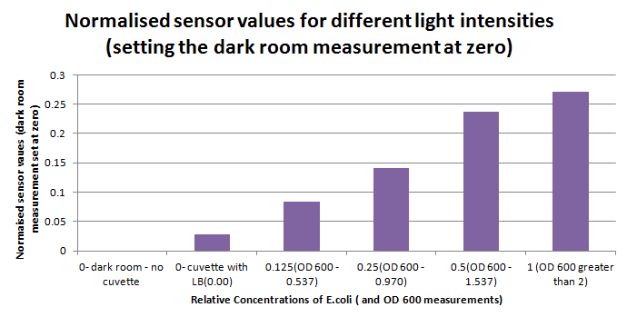
Having our instrumentation completed, as can be seen in our Instrumentation (Biologger) page, the sensitivity of the sensor placed in the right position was tested using a dilution series of luciferase-producing E.coli. 20ml Cultures were grown overnight from single colonies. The cultures were induced with 40ul of 1.5M arabinose (for a final concentration of 3mM). Cultures were left for 2 1/2 hours for full induction. Subsequently, a culture was pelleted and resuspended in 4ml LB. Doubling dilutions, of volume 2ml, were made from this concentrate, down to 1/8th concentration. 1ml of each 2ml dilution was analysed in each cuvette, which was placed in the cuvette holder we made ourselves. The result was very good. An almost linear relationship was obtained when data were normalised with the sensor value taken in the dark room (the latter set at zero) without using the cuvette holder (1-(sensor value/sensor value in absolute dark)), presenting the sensitivity of the sensor to different intensities of light. This behaviour was expected due to the changing offset affecting the luciferase spectrum curve at different light intensities. The offset, using our data, was calculated to be about 0.2V for each dilution. A second graph is shown which takes into account this offset (and removes it), thus showing the presence of blue frequencies. The result was as expected, as the presence of blue frequencies throughout the dilution series is not only detected, but also found to be approximately constant. The raw data of this investigation can be found in the Lab book.
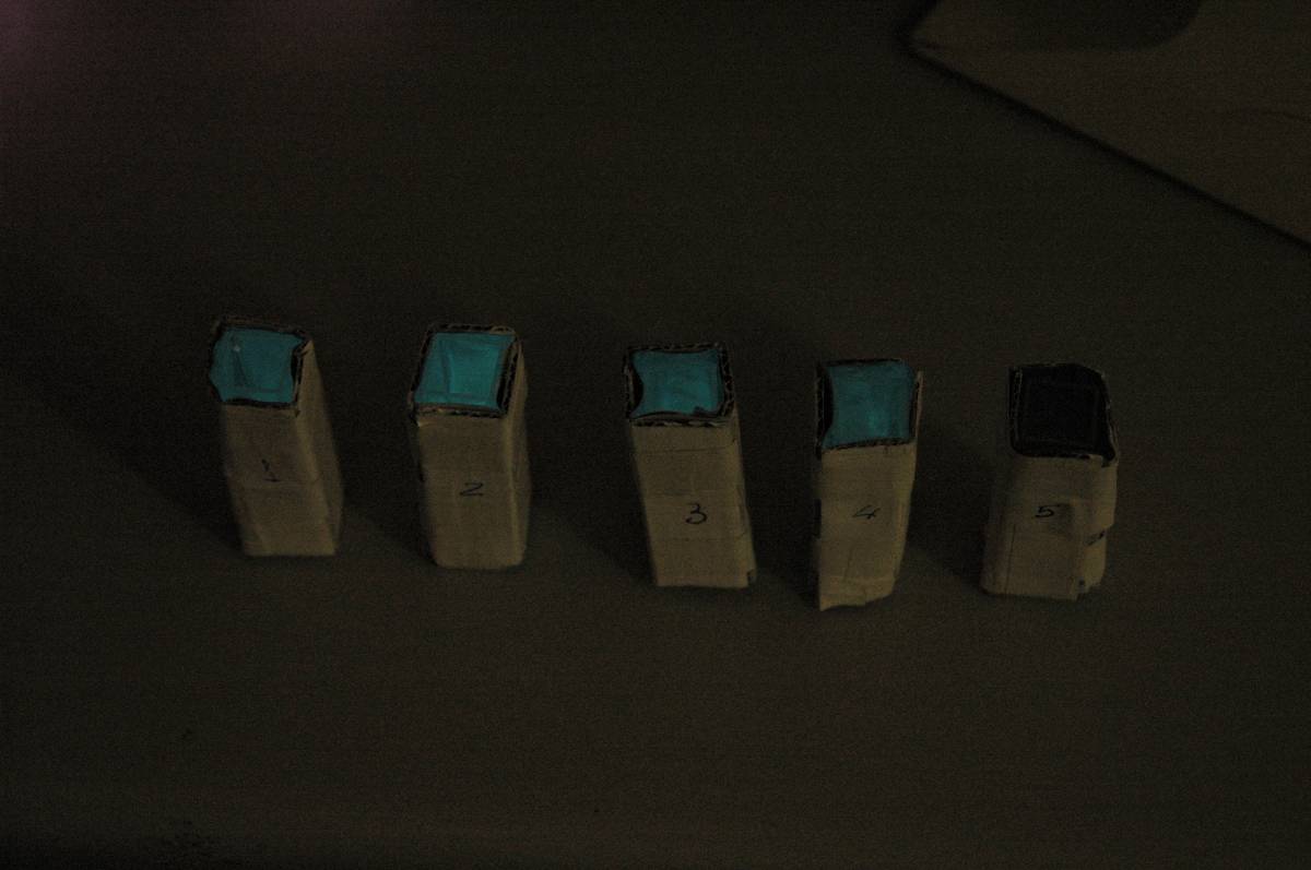
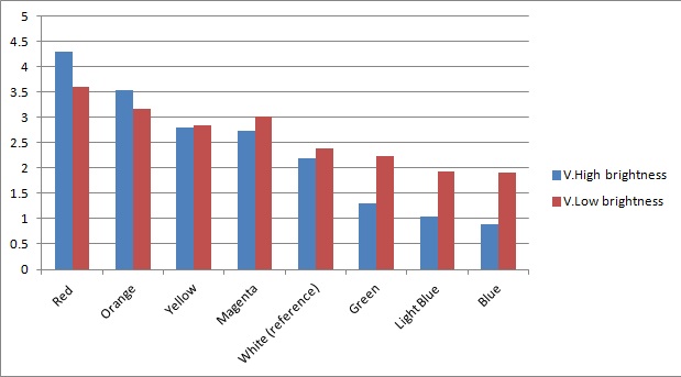
Once the sensor was tested for sensitivity, we tested that our circuitry correctly identified different frequencies (colours) of light. As can be seen below, measurements taken from orange and blue light yield values respectively above and below those from white light (our reference point). The data was taken using constant intensity of light for each case (V.High and V.Low brightness, as specified in the application). This was done with the aid of an Android phone and a specialised software application, called Color Flashlight, downloaded from the official Market.
As expected from the potential-divider design of our circuitry, orange and red frequencies caused the resistance of the LDR with the orange filter to decrease, leading to a higher voltage across the LDR with the blue filter. The opposite effect was observed with blue light. The reason that the white reference point is a bit lower than 2.5V (the expected value for a non-biased circuitry with a 5V source), is because we use resistors of total net resistance 1.67 kΩ before the blue LDR. This was done to bias the circuitry towards blue (i.e. decreasing the starting value, thus the sensor identifies always a bit more blue - this can be shown in previous graphs as well) and thus cause orange light to have a larger impact when present. This was used in an attempt to compensate for the fact that the peak at 560nm (Orange) in MOrange/luciferase fusion spectrum is lower than the one at 490 nm (Blue). Even though we did not manage to test the latter with transformed bacteria, the data collected in all the previous experiments makes us confident that the instrumentation is at least adequately functional.
As the major part of the instrumentation, the bio-electronic interface, had been made and tested, now we turned to testing the other parts of our deveoped kit. This included the mechanical chassis of the prototype, the electronic/mechatronic (sensory and motory) components, and of course the software. The overview of the finished hardware/software can be seen in our Intstrumentation (Biologger) page. Below, the videos showing our instrumentation in action can be seen.
 "
"


