 "
"
Team:UANL Mty-Mexico/Modeling/Biosensor
From 2012.igem.org
Biosensor
Our biosensor model is a continuation of the previously exposed transport and accumulation model with the addition of the production of luciferase as a function of ArsR|As concentration. In this way, we can relate the concentration of extracellular As to the production of luciferase.
ODEs
The ODEs that describe the kinetics of the biosensor modules include all the assumptions presented in the core model and the equations presented for the accumulation and transport module, along with their corresponding parameters.
Taking into account the equations from the accumulation and transport module, we introduce a generator for Luciferase:
Luciferase mRNA
\begin{equation} \large \frac{d[mRNA_{Luc}]}{dt} = \alpha _{mLuc}\cdot (pro_{ars})\cdot(\frac{k_{D1}^{h_{1}}}{k_{D1}^{h_{1}}+[ArsR]^{h_{1}}})- \delta _{mRNA_{Luc}}[mRNA_{Luc}] \end{equation}Luciferase protein
\begin{equation} \large \frac{d[Luc]}{dt} = \alpha _{pLuc}\cdot[mRNA_{Luc}]- \delta _{Luc}[Luc] \end{equation}Parameters
The parameters for the ODEs describing the production of luciferase mRNA and protein are shown in the next table.
Parameter table
|
Parameter |
Description |
Value |
References |
|
αmArsR |
Maximal transcription rate of ArsR |
3.74 nM/min |
Assumptions |
|
αmFluc |
Maximal transcription rate of Fluc |
1.40 nM/min |
Assumptions |
|
αpArsR |
Maximal translation rate of ArsR |
9.74 nM/min |
Assumptions |
|
αpFluc |
Maximal translation rate of Fluc |
2.06 nM/min |
Assumptions |
|
δmRNAArsR |
Degradation rate of ArsR mRNA |
2.16x10⁻¹ min-1 |
Assumptions, Selinger, et al. (2003) |
|
δmRNAFluc |
Degradation rate of Fluc mRNA |
3.37x10⁻² min-1 |
Assumptions, Suter, et al. (2011), Karetnivok and Lehto (2006). |
|
δArsR |
Degradation rate of ArsR |
2.31x10⁻² min-1 |
Assumptions |
|
δFluc |
Degradation rate of Fluc |
2.60x10⁻² min-1 |
Assumptions, Auld, et al. (2008) |
|
proars |
Concentration of ars promoter |
aprox. 1*plasmid copy (nM) |
Assumptions |
Simulations
For the constructed ODEs, we built a Simulink model. With the extracellular As set to zero and the initial conditions for all other variables set to zero, as well, we obtained the values for the variables ArsR and Fluc (both in protein and mRNA) at steady state and used them as initial conditions for further simulations:
mRNAs: ArsR = 2.1058 nM; Fluc = 5 nM
Proteins: ArsR = 887.7 nM; Fluc = 398.6 nM
We also set all the numerical integrators to have lower saturation limits equal to zero, to be in concordance with the mass conservation law. Here are the results for simulations at extracellular As set to 0, 0.1, 1, 5 and 10 μM (0, 100, 1000, 5000, 10000 nM).
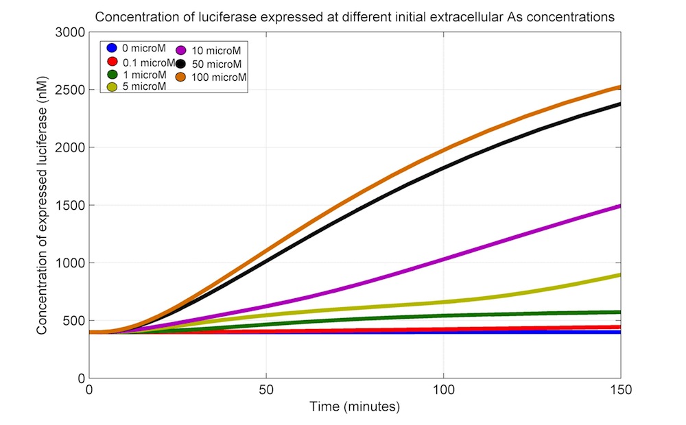 |
The last simulation shows the dynamics of the Luc production at different As concentrations; now we want to know the dynamic range of our biosensor. In order to do this, we performed simulations at varying extracellular As concentrations (ranging 0, 0.1, 1, 5, 10, 50 and 100 μM) and recorded the level of Luc at 150 min. Next, we plotted the pairs of extracellular As concentration and Luc levels at 150 min; this pairs were then fitted to a rational curve using the Matlab fitting tool, so we ended with a formula for the theoretical relation between extracellular arsenic and Luc levels at 150 min
 |
Function relating extracellular arsenic and Luc
\begin{equation} \large [Luc] = \frac{2816[As]^{2} + 316.6[As] - 607}{[As]^{2} + 10.24[As] - 3.521} \end{equation}The R2 for this equation as a regresion of the actual data was 0.998.
Simulink model: biosensor
See our simulink model here.
