"

From 2012.igem.org

Home

Team

Team Profile

Project

Parts

Modeling

Notebook Calendar Thermosensor Lactate Sensor Cre Lox

Safety

Outreach

Collaboration

Attributions

Contents 1 Introduction 2 Our Circuit 3 The Model 3.1 Mass-Action Equations 3.2 System of ODEs 3.3 Parameter Estimation 3.4 Solutions 3.5 Temperature Dependence 4 Analysis 4.1 Steady State Analysis 4.2 Bifurcation Analysis 5 Modeling our Thermosensor Library 5.1 Smith-Waterman Algorithm 5.2 Our Revised Algorithm 6 Acknowledgments

Introduction

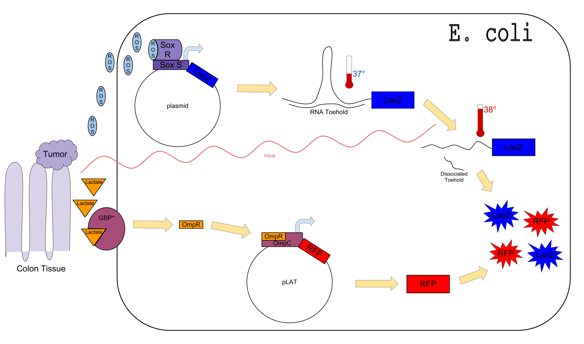
Colon cancer polyps produce high amounts of reactive oxygen species (ROS) and lactate. The high metabolic activity also causes an increase in temperature. Sensors for any one of these inputs alone would be confounded by normal physiological variation in temperature, lactate concentration, and ROS concentration. We propose a genetic circuit designed to detect higher than normal levels of all three, producing two separate outputs. There are two parts to the circuit: The first is a dual input system, using temperature and ROS as inputs to produce an output (LacZ). The second is a single input system, using lactate to produce GFP. Our analysis focuses on the dual input system which senses ROS and temperature to produce LacZ.

Insert picture of model here

In order to model our system, we have undertaken three main tasks:

1) Create a model using Mass-Action Enzyme Kinematics

2) Analyze this model using computational methods

3) Create an algorithm to predict the structure of our RNA thermosensors

We will start by describing the reactions within our circuit and then by creating a system of differential equations from the reaction sequence.

Our Circuit

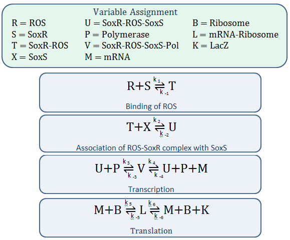
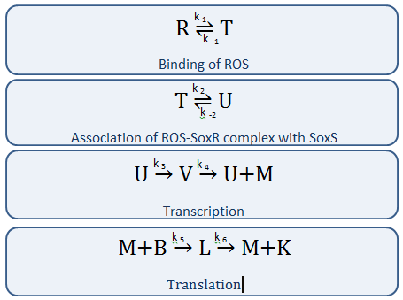
The diagram above depicts the inner workings of our circuit created within E. Coli. The following chemical equations depict the pathway, involving our dual-input system:

The Model

The following describes our attempts to create a model which can predict the behavior of our system. Although it is certainly not 100% accurate, it can, to some extent, predict the outcome for a determined set of initial conditions.

Mass-Action Equations

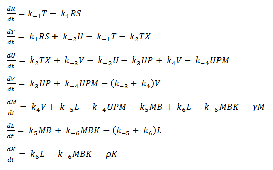
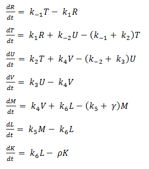
Using mass-action kinetics, we wrote the chemical equations as a system of differential equations.

The k constants, as shown above, represent reaction rates and

System of ODEs

As it is, the system is too complicated for us to analyze, so we hereby make a few assumptions to simplify.

• Eliminating Constant Variables

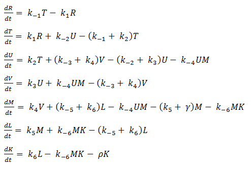
In our model, SoxR (S), SoxS (X), Polymerase (P), and Ribosome (B) never change concentration and we assume that they are in excess compared to the other species. Therefore, we eliminate them from the model, simply combining them with the other constants.

• Reverse Reaction Assumption

The last two chemical equations represent transcription and translation, respectively, and these two processes are assumed to have a forward reaction only. Therefore, we set all k values for the reverse reactions equal to zero.

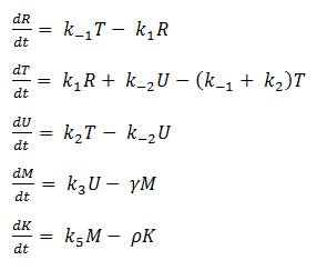
Thus we are left with the set of equations shown below.

• Quasi Steady State Assumption

We assume that the concentration of the intermediates of transcription and translation do not change on the time-scale of mRNA and protein formation, therefore, we set

We are then left with the following set of equations:

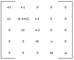
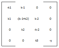
We define the matrix A to be:

And the vector v to be:

Therefore, our system is simply: v ' = A * v

Parameter Estimation

Most of the parameters were not readily available in databases, but we were able to figure out reasonable values for each one. The rate of nucleotide addition in transcription is about 60 per second and the rate of amino acid addition in translation is about 20 per second. Our mRNA is approximately 3200 nucleotides long, therefore an appropriate value for k3 and k5 was found by dividing 60 by 3200. Thus k3 = 0.0187/sec. Noting that in E. Coli the lifespan of mRNA is about 60 seconds and the lifetime of protein is approximately 1 day, we find that y = .0167/sec and p = 0/sec. Because p = 0, this automatically reduces our system of differential equations, because we find that the concentration of protein is now only dependent on the concentration of mRNA, in a linear fashion. We can therefore say that the protein follows the mRNA: whatever the mRNA (M) does in the model, the protein (K) will do as well. Our matrix A then becomes:

From the work of [http://jaguar.biologie.hu-berlin.de/~wolfram/data/ibsb2007_Borger_et_al.pdf Borger et. al 2007] we find that kinetic rate constants for reactions involving only reactants can be described by a Gaussian distribution with a median of 0.14. Kinetic rate constants for reactions involving reactants and enzymes have a Gaussian distribution with a median of 6.0. The first of our chemical reactions is viewed as an interaction between reactants and the second as an enzyme reaction. Thus, to get values for k1 and k-1 and for k2 and k-2 we created a Gaussian distribution around the appropriate median and chose randomly from this distribution.

We chose the initial concentration of ROS to be .001 M (even smaller values may be expected in the body) and the initial concentration of the other 3 species to be 0 M.

Solutions

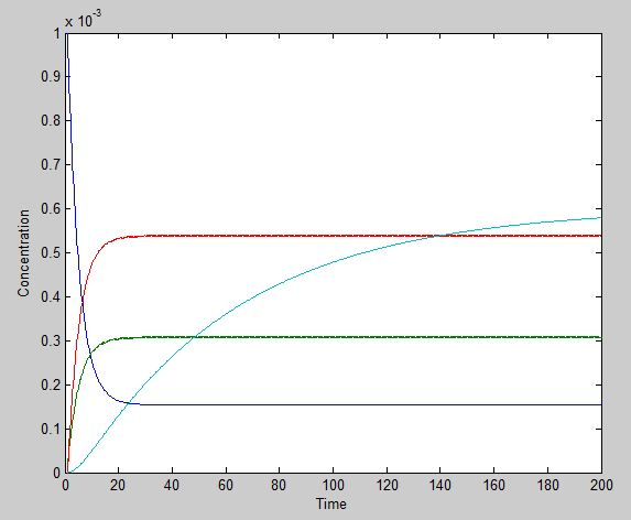
Using the ode23 solver in Matlab we are able to graph the solutions to our system of differential equations.

We chose a 200 second time interval. The dark blue line is the time-evolution of ROS concentration and the light blue shows the change in mRNA concentration over time. The other two lines represent the intermediates. The model presents a typical, ideal situation that fits our system well: as time increases, the ROS concentration decreases, leveling off. The concentration of mRNA increases with time, also leveling off and the concentration of the two intermediate species, T and U, increase and level off even faster. Please note that it is assumed that once the ROS enters the cell, it is degraded and not used again.

Temperature Dependence

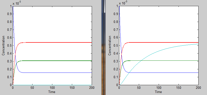
In order to accurately model the system, we also need to take into account the temperature dependence of the thermosensors. This introduces another variable into the system: temperature. We did this by multiplying the rate constant k3 by a heaviside function defined as follows:

This essentially turns on the thermosensor at the appropriate temperature. Applying the heaviside function, the solutions when T < 35˚C will be different than those when T > 35˚C. The graph on the left shows the solutions when T < 35˚C and the graph on the right shows the solutions when T > 35˚C. It is apparent that only the mRNA concentration is affected.

Analysis

Steady State Analysis

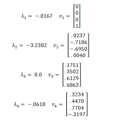
The eigenvalues and eigenvectors of A are:

Because the third eigenvalue is 0 this tells us that there is a line of steady states defined by the third eigenvector, v3. The other 3 eigenvalues are negative, representing stable solutions which will converge to the steady state.

Bifurcation Analysis

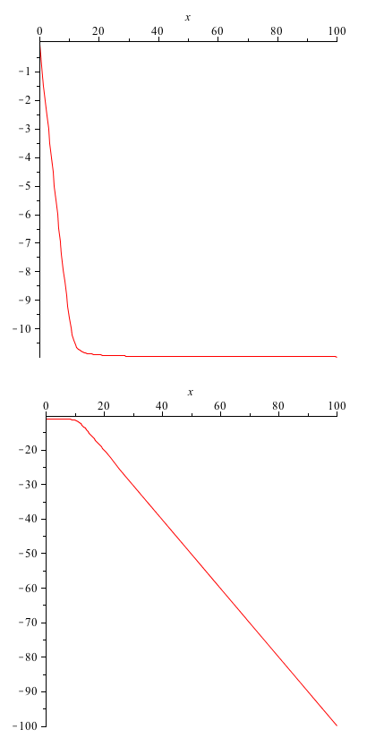
One of the rate constants we are most interested in is the value for the forward rate of the first reaction. This gives us information about the binding of ROS to the SoxR membrane protein. Here we provide a quick analysis of this constant. Taking the A matrix we put in values for each constant except k1. Then, using Maple, we found the eigenvalues of the matrix, as functions of k1. The first and third eigenvalues remained the exact same (they weren't dependent on k1 at all), but the second and fourth were given to us as functions of k1. These we plotted.

y-axis: eigenvalue x-axis: varying parameter value (k1)

From these graphs we do not see a bifurcation (the eigenvalues always remain negative). This simply means that we don't have very much control over the system, when working with the k1 parameter.

Modeling our Thermosensor Library

Herein we provide detailed information about our library of thermosensors and describe our attempt to model the secondary structure of the RNA hairpins. We provide a description of an algorithm we developed, similar to the Smith-Waterman algorithm.

Smith-Waterman Algorithm

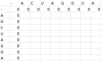
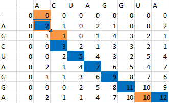
The Smith-Waterman Algorithm is a simple process used to perform sequence alignment. To demonstrate how the algorithm works, we will use these two sequences:

• ACUAGGUA
• AGCUAGGA

First one sequence is placed in the first row of a grid, skipping the first two entries in the row. The second is likewise placed in the first column, skipping the first two entries in the column. Zeros are then placed in row 2 and column 2.

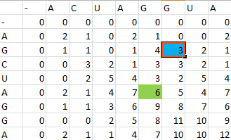
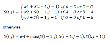
Then, a scoring matrix, S is created according to the following rules:

For example S(4,8) in the blue was obtained by adding 2 to the number in the entry in the upper left-hand corner. S(7,7) was obtained by adding -1 to the max of the 3 numbers above, on the upper left-hand corner, and to the left of it.

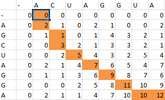
Once the scoring matrix has been completed, starting in the bottom right corner, a path is chosen, picking the largest numbers (only numbers to the left, above or up and to the left can be chosen), until the path arrives back at a zero. When a number above or to the left is the same as the number on the diagonal, the number above or to the left is to be chosen first.

The resulting path spells out the proper alignment of the two sequences. Squares alone in their row and column represent an alignment and when two or more squares share the same column or row, the one closest to the bottom right corner is the one that represents the alignment. The other squares represent deletions or insertions. For our example, the final alignment is shown in the blue.

Thus the alignment of the two sequences would be:

• A--CUAGGUA
• AGCUAGG--A

Source: [http://docencia.ac.upc.edu/master/AMPP/slides/ampp_sw_presentation.pdf Ayguade et. al 2007]

Our Revised Algorithm

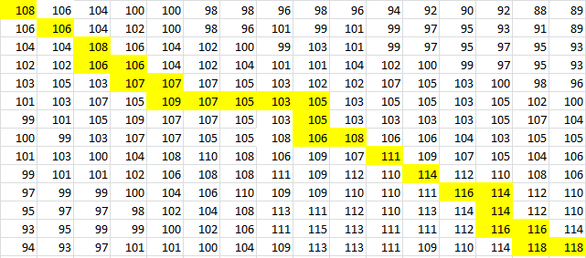
Using the same ideas applied in the Smith-Waterman method, we created an algorithm to model the secondary structure of our RNA thermosensors. The main difference is that we are aligning one side of an RNA sequence with its other side and we are not working with two separate sequences. Thus, we create a similar scoring matrix by placing the RNA sequence along the top row (skipping the first 2 entries) and by placing the reverse of the RNA sequence down the first column (also skipping the first 2 entries).

We then assign priorities in this way:

The if statements refer to the alignment of different base pairs. Here, w1, w2, w3 and w4 are weights that we assigned unique to our library of thermosensors.

• w1 = 3
• w2 = 2
• w3 = 1
• w4 = -2

To provide an example, we will use TSA, the wild-type thermosensor.

The sequence is:

uuuagcgugacuuucuuucaacagcuaacaauuguuguuacugccuaauguuuuuaggguauuuuaaaaaagggcgauaaaaaacgauuggaggaugagacaugaacgcucaa

After placing the forward sequence along the top row and the reverse sequence down the first column, we start at the very bottom right corner and proceed to find our way back, following the path that gives us the largest values. The rules for our algorithm are as follows:

• 1) To go from one entry to another, the largest of the three values in the entries to the left, above and in the left-hand corner is picked.
• 2) If the largest value is present twice, once in the corner and once to the left or above, always choose to move to the left or above before moving to the corner entry and then only move to the corner entry if it is the largest number for the next pick.
• 3) If the largest value is present in both the left entry and the one above (3 times if present in the corner entry as well), choose the one which will give the largest number in the next pick, and so on.
• 4) Continue on this path until the entry S(i,j) has been reached where i+j = n | n = total number of bases in the RNA sequence being analyzed. This represents the point where the thermosensor turns around. To continue would be, essentially, going back the way you came.
• 5) Then, pick every entry which is connected to another entry only by a corner. Discard all entries which sit in an irregular position. There are 2 types of irregular positions. First, if an entry in the lower right hand corner is less than the entry in the upper left hand corner, discard the entry in the lower right hand corner. Second, if an entry stands alone, not connected to any other entries, discard that entry. See figure for an example.
• 6) Last, because of the hairpin loop, we eliminate the last two bonds, where the loop occurs, if the algorithm did predict bonding in that region.

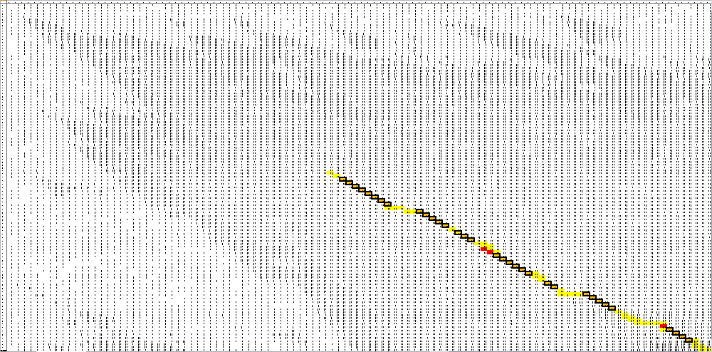
Here is the final path:

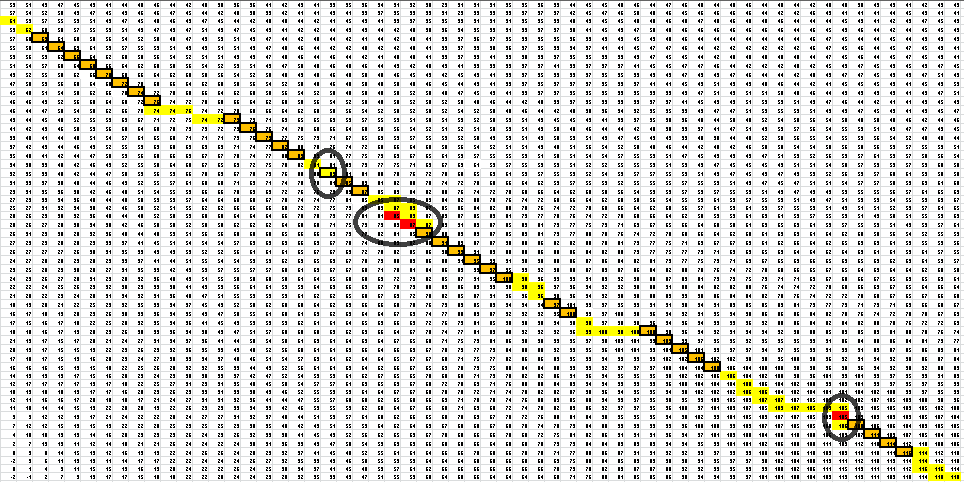
Here is a breakdown of the color scheme:

• Yellow is the path determined by our algorithm
• The dark-outlined boxes are the entries chosen by our algorithm-these determine the bonding patterns
• Red are the actual bonding patterns observed in the secondary structure of TSA
• Orange is where the actual bonding patterns fall on the same path predicted by our algorithm
• Ovals indicate regions where our algorithm differs from the rnafold program in Matlab

And for a look at the entire scoring matrix:

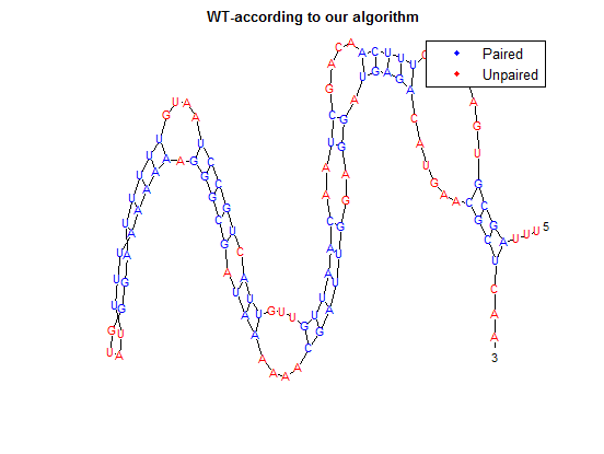
Once this path is determined, it is then converted into a series of dots and parenthesis which represent the bonding in the RNA structure. The bonding pattern determined by our algorithm is:

...((((........(((((....((..((((((...(((.(((((....((((((((....)))))))).))))).)))....))))))..)).)))))......))))...

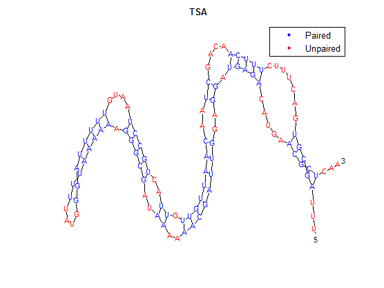
The bonding pattern predicted by rnafold in Matlab is:

...(((((.......(((((....((..((((((((.((..(((((....((((((((....)))))))).)))))..))..))))))))..)).))))).....)))))...

The secondary structure, according to our algorithm is shown below, followed by the secondary structure determined by Matlab.

We did not perform this algorithm by hand, instead we wrote a program for it in Matlab. This algorithm has not been tested with other RNA sequences outside of our library of thermosensors. It is useful because we can ues it to predict the structures of our thermosensors and, in the future, other thermosensors that are made by mutating the current ones.

Acknowledgments

The modeling for this project was performed by John Shumway. A special thanks to Dr. John Dallon in the BYU Math Department for help with the system analysis and Eric Jones, a member of the BYU iGEM team for help with the ODEs.