Team:Colombia/Notebook/Journal
From 2012.igem.org
The Journal
Chitinase
To determine which chitinase is going to be used, we screened chitinase from 3 different species since the chitinase of different Vibrio spp. was not suitable or the strain was found (Alivibrio fischeri ES114, Alivibrio fischeri M11):
- Arabidopsis thaliana
- Colletotrichum spp.
- Trichoderma sbpp.
For each one we obtained accesion numbers:
- Arabidopsis thaliana: [http://www.ncbi.nlm.nih.gov/nuccore/AY099810.2 AY099810.2]
- Colletotrichum spp. : [http://www.ncbi.nlm.nih.gov/nucest/GW342409.1 GW342409.1]
- Trichoderma spp. : [http://www.ncbi.nlm.nih.gov/nucest/BM077089.2 BM077089.2]
Each one was tested using codon usage for bacteria (Translation table 11) to determine if the chitinase could be used. All of the sequences were suitable for use.
We selected Colletotrichum spp. and Trichoderma spp. sequences to design primers.
Primers
- Colletotrichum spp. :
- Trichoderma spp. :
Ralstonia solanacearum
June 8
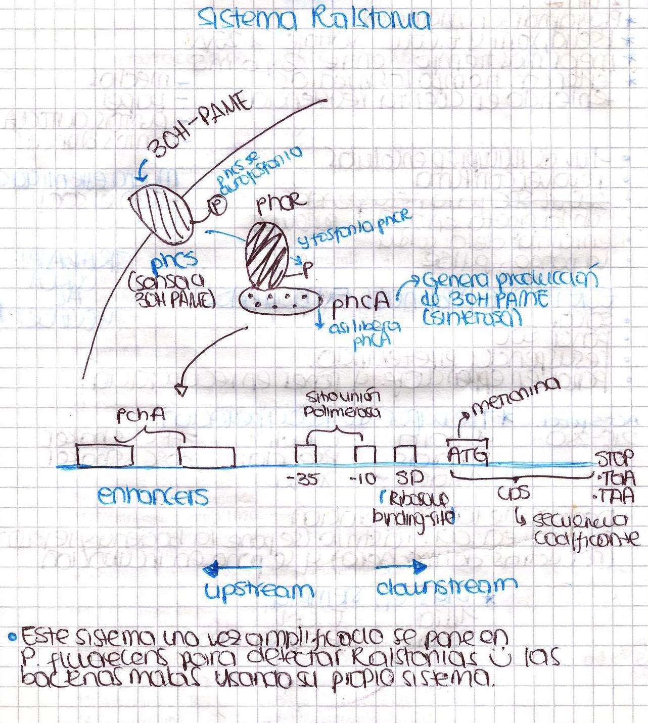
Today we had our first meeting! We introduced ourselves and basically talked about Ralstonia solanacearum detection system and made a little research to find a proper culture medium in order to grow our bacteria. Here is a little sketch we made.
June 12
We decided to prepare Casamino acid-Peptone-Glucose (CPG) media, which is a rich medium that provides everything that Ralstonia solanacearum needs to grow and we have all the components in the lab. This is the recipe for 1L of CPG:
| Reactives | Amount (g) |
|---|---|
| Casamino acid | 1 |
| Peptone | 10 |
| Glucose | 5 |
| Agar | 15 |
June 13
We grew a Ralstonia solanacearum strain in solid medium from the REVCO, it belongs to the phytopathogen bacteria strain store at the LAMFU, it will fully grow in 2 days, so we have to wait until then…everything is pretty easy so far.
June 15
We were going to extract DNA from Ralstonia tomorrow, so today we spent a lot of time preparing all the solutions needed. Ralstonia strain didn’t grow, we are kind of upset. We also designed the primers to amplify the promoter of xpsR(PxpsR) We used the sequence of Ralstonia solanacearum AW (gi:3132834)as this promoter sequence has been previously characterized by [http://www.ncbi.nlm.nih.gov/pubmed/9573161 Huang et al. in 1998.]
June 16
Today is a new day, we decided to grow a different accession of Ralstonia solanacearum and see what happens. Hopes up!
June 18
Our bacterium is alive! it doesnt matter that today’s hollyday anymore and we are at lab….We are finally extracting DNA tomorrow, so we inoculated 5 ml of liquid CPG with a few colonies from the solid culture and left it growing ON.
June 19
Today was DNA extraction day! We used Xam’s DNA extraction protocol(see protocols) and here it is, our Ralstonia’s DNA, we think is a little bit degraded but still amplifiable…
June 20
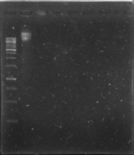
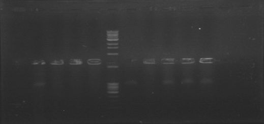
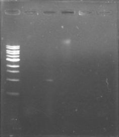
Today we were supposed to amplify all the genes for the detection system but PxpsR (those primers haven’t arrive yet). We used Fermentas Pfu (see protocols) and the Ta for each gene was calculated taking the lower primer Tm of each couple and subtracting it 2 degrees (phcS=61°C, phcR=57°C, phcA=54°C). Nonetheless, none amplified. We are no longer sure if the primers anneal in all Ralstonia strains, we haven’t consider that before.
June 21
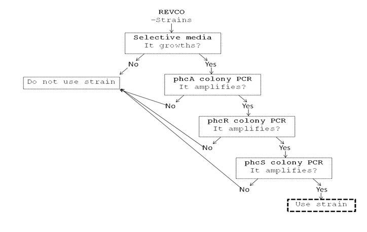
We performed a primer search in NCBI and confirmed our suspects … there are some base changes at the 3’ of our primers in the sequence of different strains of R. solanacearum…that will explain why it didn’t amplified a thing yesterday. The most conserved sequence appear to be PxpsR and then phcA, so, while PxpsR primers arrive, we will perform a screening of differtent Ralstonia solanacearum strains using phcA, then we will try to amplify the other genes from positive strains. Here is our decision tree.
June 22
Today we prepared the selective media for the screening; we had to make substantial variations due to a lack of compounds in our lab. This was the final composition:
| Reactives | Amount |
|---|---|
| Mannitol | 1g |
| Na2HPO4 | 3g |
| KH2PO4 | 3g |
| NH4Cl | 1g |
| MgSO4 | 0.25g |
| FeSO4 | 5mg |
| Crystal Violet | 3mg |
| Cycloheximide | 5mg |
| Chloramphenicol | 1mg |
| Bacitracine | 0.25mg |
| Agar | 15g |
| Distilled water | 1L |
June 24
We decided to make a pilot experiment in order to standardize the conditions of phcA amplification before starting with the massive screening . We choose #37 strain randomly for the standardization.
June 26
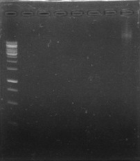
In order to standardize the conditions of phcA amplification before starting with the massive screening , we determine the annealing temperature (71°C) by performing an in silico PCR (FAST PCR) and used that temperature to calculate a temperature gradient (form 64 to 71), reactions were carried out with and without DMSO. The results weren’t expected, none of the temperatures amplified.
June 27
We perfomed phcA PCRs using boiling from the solid culture as a source of DNA. The results remained the same. Due to results we decided to change of strains and we grew on solid 3 new accessions.
June 28
The primers for the promoter of xpsR finally arrived! We intented to amplify this promoter due to the conservation of the secuence using the DNA previously extracted and using a Ta of 46°C. We expected a band of 389pb but we couldn’t even see primer dimmers.
June 29
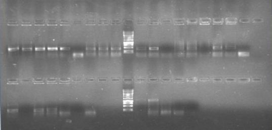
We are finally in the right direction! Today we massively performed PCR of the 3 new strains to amplify PxpsR using a temperature gradient (form 45 to 69). All but one seemed to amplify in almost all the temperatures! Thats the one!!
July 3
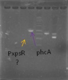
Now that we know that PxpsR amplifies, we continue following our decision tree and try with phcA, we only used the strains where PxpsR amplified. We used the temperature gradient previously named for phcA. Fortunately for us all the strains were positive.
July 5
Today we tried to amplify both PxpsR and phcA with Pfu in order to clone in the backbone (pBS1C3), as both genes had amplified previously at 64°C we choose that temperature as the Ta, allthough it didn’t work for PxpsR.
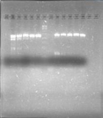
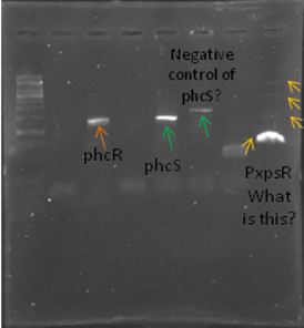
We also tried to amplify phcR and phcS using a gradient temperature from 57 to 67 with the strain #75 that always amplified better than the others. Surprisingly both genes amplified just fine at all temperatures, but there was double band, even in the highest temperatures, so we will have to cut band after amplifying with Pfu.
Finally we digested (see protocols) phcA with EcoRI and SpeI, and the backbone with EcoRI, SpeI and DpnI, and we also ligated (see protocols) with T4 ligase through the night.
July 6
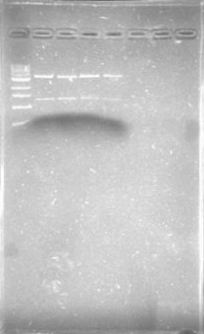
Today we amplified PxpsR, phcR and phcS with Pfu, we used the lowest temperature for PxpsR (45°C), but once again PxpsR didn’t amplify as we expected (more than 1 band).
We also transformed by electroporation (see protocols) the ligation of phcA into the backbone, we hope to see colonies in the morning.
July 7
Nothing grew into the plate! We are not sure if the restriction enzymes aren’t working well or the T4 ligase is failing… We tested the restriction enzymes using as target the salicylic acid biobrick, we performed different combinations of enzymes (PstI-EcoRI, EcoRI-SpeI, XbaI-PstI, SpeI-XbaI) that excises a fragment of 1500bp. Conclusion: Everything seems to be fine with the enzymes, it must be the T4 ligase.
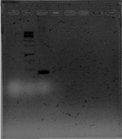
We also repeated the PCR for PxpsR this time using as Ta 50°C, it amplified!
July 10
We are back in the game, we have a different ligase and we are making new electrocompetent cells!
July 12
Today we are going to transform phcA+BB, phcR+BB, phcR+BB and PxpsR+BB in our just prepared competent cells. Tomorrow we will make passes of the colonies.
July 13
There are not colonies in the plates…maybe the cells aren’t that competent, we will try again with other cells…
Mathematical Models
Up to June 6
Up to June 6 we organized the variables and parameters of our design, formulated the differential equations for each of the molecules of the model and set out to look for parameter values in literature. This link is the depurated version summary of the model that should be included in the Modeling section of the wiki.
July 3
Today’s subject was the parameters to be used at differential equations that had been previously developed. In order to do this, a set of parameters, to be searched from different sources, had been assigned to each member of the team. According to the results obtained it was established to categorize each group in a range as it is shown below:
- α group: Since no value was found it would be supposed at first that all values are the same.
- γ group: For this parameters, Gabriel proposed to bear in mind the lifetime of a E. coli. As a backup, rates of normal destruction in proteins (in general) and salicylic acid could be looked for.
- Kinetic constants of reaction: We will focus on ChiA and look for any number of cellular kinetic trying to find a maximum.
- βx group: Search concentrations of the most produced protein in E. coli, RubisCo and the least produced to establish a range.
- Parameters of export and import: To reference export and import rates of any protein and then try to establish a range.
July 10
The following document has all the information we could find about parameter approximate values. It is in spanish, but it should be translated and included in the Modeling section of the wiki. File.
Our first matlab code was written today too. It is a two file code:
Code for ecuaDif.m
%Codigo que contiene todas las ecuaciones diferenciales de los procesos
%dados en los 3 plasmidos
function y=ecuaDif(t,v) % Funcion que devuelve un vector y con todas las ecuaciones, tiene como
parametro un vector con los parametros y un vector v
%las variables.
QQ=10;

%------ Variables%------

Ao=v(1); %Cocentration of chitinase outside the cell
Ai=v(2); %Concentration of chitinase inside the cell
P=v(3);  %Concentration of chitiporin
C=v(4);  %Concentratio of chitin binding protein (CBP)
CS=v(5); %Concentration the complex CBP-s
R=v(6);  %Concentration of LuxR
Ii=v(7); %Concentration of LuxI inside the cell
Io=v(8); %Concentration of LuI outsied the cell
IR=v(9); %Concentration of the complex LuxI-LuxR
CI=v(10);%Concentration of the protein CI
HA=v(11);%Concentration of HipA7
HB=v(12);%Concnetratio of HipB
AS=v(13);%Concentration of salicylic acid
Q=v(14); %Concentratio of quitin monomers
                          %----Parameters----%

%All the parameter came in a vector given by other function.

alfA=0.4;      %Basal concentration of Chitinase inside the cell (micromolar)
alfP=0.4;      %Basal concnetration of chitoporin
alfC=0.4 ;      %Basal concentration of the CBP
alfR=0.4;      %Basal concentration of LuxR
alfI=0.4;      %Basal concentration of LuxI
alfCI=0.4;     %Basal concentration of CI
alfHA=0.4;     %Basal concnetration of HipA7
alfHB=0.4;     %Basal concnetration of HipB
alfAS=0.4;    %Basal concnetration of Salycilic acid


gammaA=0.01;    %Degradation of Chitinase inside the cell
gammaP=0.01;    %Degradation of chitoporin
gammaC=0.01;    %Degradation concentration of the CBP
gammaR=0.01;    %Degradation of LuxR
gammaI=0.01;    %Degradation of LuxI
gammaCI=0.01;   %Degradation of CI
gammaHA=0.01;   %Degradation of HipA7
gammaHB=0.01;   %Degradation of HipB
gammaAS=0.01;   %Dergradation of Salycilic acid
gammaCS=0.01;   %Degradation of the complex CS


mCS=5;      %Kinetic constant for the formation of the complex CS
mCSQ=5;     %Kinetic constant of the reaction of the complex CS with the chitin
mAQQ=5;     %Kinetic constant for the reaction of the chitinase and th chitin
mIR=5;      %Kinetic constant for the formation of the complex LuxILuxR
mI=5;       %Constant that represent the union of the complex LuxILuxR with the promoter
mHAHB=5;    %Kinetic constant for the inhibition of HipA7

betaP=10;    %Max production of the chitoporin
betaA=10;    %Max production of chitinase
betaI=10;    %Max production of LuxI
betaCI=10;   %Max production of CI
betaHB=10;   %Max peoduction of HipB
betaHA=10;   %Max production of HipA7
betaAS=10;   %Max production of Salicylic acid

kS=1;      %Constant k of the hill ecuation for the promoter promoted by S
kIR=0.5;     %Constant k of the hill equiation for the promorer prmoted by the complex luxIluxR
kCI=0.1;     %Cosntant k of the hill equation for the promoter promoted by CI


hS=1;     %Hill constant for the promoters promoted by S
hIR=3;    %Hill constant for the promoter promoted by the complex IR
hCI=2.3;    %Hill constant fot the promoter CI


eA=0.5;     %Exportation factor of the chitinase
jQ=0.8;     %Importation factor of the chitin monomers
deltaA=0.2; %Difusion factor of the chinitanse outside the cell

eI=0.5;    %Exportation factor of LuxI
jI=0.8;    %Importation factor of LuxI
deltaI=0.2;%Difusion of LuxI outside the cell

Stotal= 1;  %Total concentration of the sensor in the cell

numcel=100;   %number of cells


                                %---Equations---%

S=Stotal-CS;


dC=alfC- gammaC*C - mCS*C*S; %Change of CBP

dCS=mCS*C*S- mCSQ*CS*Q-gammaCS*CS;  %Change of the complex CS

dP=alfP - gammaP*P + (betaP*(S^hS))/(kS+(S^hS));%Change of chitoporin

dAi=alfA- gammaA*Ai+ (betaA*(S^hS))/(kS+(S^hS))- eA*Ai; %Change of chitinase inside the cell

dAo= eA*Ai-deltaA*Ao- mAQQ*Ao*QQ; %Change of chitinase outside the cell

dQ= jQ*P*(mAQQ*QQ*Ao)-mCSQ*CS*Q; %Change of chitin monomer inside the cell

dIi= alfI+ (betaI*(S^hS))/(kS+(S^hS)) -gammaI*Ii +jI*Io- eI*Ii- mIR*Ii*R; %Change of LuxI inside the cell

dIo= numcel*(eI*Ii-jI*Io)-deltaI*Io; %Change of LuxI outside the cell

dIR= mIR*Ii*R - mI*IR;  %Change of the complex LuxI luxR

dR= alfR-gammaR*R -mIR*Ii*R; %Change of LuxR

dCI= alfCI -gammaCI*CI+ (betaCI*(CI^hCI))/(kCI+(CI^hCI))+(betaCI*(IR^hIR))/(kIR+(IR^hIR));%Change of CI

dHB=alfHB-gammaHB*HB+(betaHB*(CI^hCI))/(kCI+(CI^hCI))+(betaHB*(IR^hIR))/(kIR+(IR^hIR))-mHAHB*HA^2*HB^2; %Chanche of HipB

dHA=alfHA-gammaHA*HA+ (betaHA*(CI^hCI))/(kCI+(CI^hCI))-mHAHB*HA^2*HB^2; %Change of HipA7

dAS=alfAS-gammaAS*AS +(betaAS*(CI^hCI))/(kCI+(CI^hCI));  %Change of Salicylic acid


y1(1)=dC;
y1(2)=dCS;
y1(3)=dP;
y1(4)=dAi;
y1(5)=dAo;
y1(6)=dQ;
y1(7)=dIi;
y1(8)=dIo;
y1(9)=dIR;
y1(10)=dR;
y1(11)=dCI;
y1(12)=dHB;
y1(13)=dHA;
y1(14)=dAS;
y=y1';
end
MATLAB script for solvEqua.m
%File that solves the differential equations and graphs them
h=1000; %Tiempo maximo
Chi=zeros(1,h); %Vector que almacena la concentracion de quitina
t=0:0.1:h; %Vector tiempo
conInd=[0.4,0.4 0.4,0.4,0.4,0.4,0.4,0.4,0.4,0.4,0.4,0.4,0.4,0.4];
for j=1:h-1
  if j<900
      Chi(1,j)=10;
  else
      Chi(1,j)=0;
  end
end
[T Y] =ode45(@ecuaDif,[0 h],conInd);

C=Y(:,1);

for i = 1:length(C)
   if C(i) < 0
       C(i) = 0;
   end
end
CS=Y(:,2);
P=Y(:,3);
Ai=Y(:,4);
Ao=Y(:,5);
Q=Y(:,6);
Ii=Y(:,7);
Io=Y(:,8);
IR=Y(:,9);
R=Y(:,10);
CI=Y(:,11);
HB=Y(:,12);
HA=Y(:,13);
AS=Y(:,14);
subplot(14,1,1); plot (T,C,T,CS,T,P,T,Ai,T,Ao,T,Q)
subplot(4,1,2); plot (T,R,T,Ii,T,Io,T,IR)
subplot(4,1,3); plot (T,CI,T,HA,T,HB)
subplot(4,1,4); plot (T,AS)
July 12
We had little luck graphing the code we wrote before. It seems we need to many specifications and restrictions to just use the ode function so it seemed we had to write the differential equation solver method ourselves.
We modified the ecuaDif.m file so that it may receive a chitin pulse:
if (t<(0.1) || t>0.3)
    QQ=0;
else
    QQ=1;
end
We also came up with a 4th order Runge-Kutta method for the solution of differential equations:
Code for solvEquaRK.m
%File that solves the differential equations and graphs them

h=0.44; %Tiempo maximo

t=0:0.1:h; %Vector tiempo

conInd=[0.02,0.001,0.002,0.002,0.02,0.002,0.001,0,0.001,0.04,0.003,0.04,0.04,0.02];


m=h/100; %Longitud de paso [s]
l=(0:m:h)'; %Vector de longitudes
x=zeros(length(l),length(conInd)); %Matriz de variables, en las columnas varia
                                     %la variable y en las filas varia la longitud
QQ=zeros(1,length(l));

x(1,:)=conInd;

for k=1:length(l)-1
   xk=x(k,:); %Captura de la ultima posicion de la matirz, es decir, los
   %valores actuales de las variables

   k1=ecuaDif(l(k),xk); %Primera pendiente del metodo de RK4
   k2=ecuaDif(l(k)+m/2,xk+(m/2*k1)'); %Segunda pendiente del metodo de RK4
   k3=ecuaDif(l(k)+m/2,xk+(m/2*k2)'); %Tercera pendiente del metodo de RK4
   k4=ecuaDif(l(k)+m,xk+(m*k3)'); %Cuarta pendiente del metodo de RK4

   xk1=xk+m/6*(k1+2*k2+2*k3+k4)'; %Calculo de nuevos valores para las
                                   %variables

   x(k+1,:)=xk1; %Actualizacion del nuevo vector de variables en la matriz


end

for j=1:length(l)

   if (l(j)<(0.1) || l(j)>(0.3))

       QQ(j)=0;

   else

       QQ(j)=1;


   end


end

C=x(:,1);
CS=x(:,2);
P=x(:,3);
Ai=x(:,4);
Ao=x(:,5);
Q=x(:,6);
Ii=x(:,7);
Io=x(:,8);
IR=x(:,9);
R=x(:,10);
CI=x(:,11);
HB=x(:,12);
HA=x(:,13);
AS=x(:,14);


figure(1)
plot (l,QQ,l,C,l,CS,l,P,l,Ai,l,Ao,l,Q)
 legend('QQ','C','CS','P','Ai','Ao','Q')

figure(2)
 plot (l,QQ,l,R,l,Ii,l,Io,l,IR)
 legend('QQ','R','Ii','Io','IR')

figure(3)
 plot (l,QQ,l,CI,l,HA,l,HB)
 legend('QQ','CI','HA','HB')

figure(4)
 plot (l,QQ,l,AS)
 legend('QQ','Acido Salicilico')
We found three more problems with this code:
- As with the ode function, graph solutions work until 0.44 time units.
- Some graphs show negative numbers, which should not be possible. It seems, however, to be solved using appropriate parameters.
- First results show that CI and salicylic acid concentration do not depend heavily in chitin concentration. We have to check it there is a mistake with our differential equations or whether we should change aspects of the design.
July 16
The following is the July 10 entry all translated and ready. Again, it should be posted in the modelling section of the site.
During this meeting there were determined the ranges in which each group of parameters can be found. For this, there were used different sources, obtaining the results shown below:
iGEM parameters determination
1. Basal levels of the protein: For this value, it will be assumed the same for all proteins. Range: 0-0.8µM Value taken from: http://bionumbers.hms.harvard.edu/bionumber.aspx?&id=104520&ver=10&trm=protein Where there is an average level, the lowest levels on that range were taken, since the concentration is basal. 2. Protein degradation: For all the proteins is assumed in the same way.
Range: 0-0.02sec-1
Degradation constant for RubisCo, maybe is needed to include in the constant the cell division value.
Taken from: http://www.tesisenred.net/bitstream/handle/10803/9518/marin.pdf?sequence=1
3. Reaction constant (association): Each of the kinetic constants are independent from each other.
Range: 0.1-10µM-1sec-1 Range was taken from: http://www.biokin.com/dynafit/scripting/html/node23.html#SECTION00431000000000000000
4. Maximum cell concentration (β Hill): Having in mind that RubisCo concentration is 20 times more than a normal protein, and the average range of protein concentration in the cell, we have: Range: 1.4-20µM Taken from: http://bionumbers.hms.harvard.edu/bionumber.aspx?&id=107431&ver=1&trm=rubisco http://bionumbers.hms.harvard.edu/bionumber.aspx?&id=104520&ver=10&trm=protein
5. Hill coefficient k: As it is the concentration to the maximum expression, the minimum value was taken from a paper where there had been calculated the parameters for CI and the maximum value was half of the maximum concentration calculated previously.
Range: 0.05-10µM Taken from: Gene Regulation at the Single-Cell Level. Nitzan Rosenfeld,Jonathan W. Young, Uri Alon, Peter S. Swain, Michael B. Elowitz. Science 307, 1962 (2005);
6. Hill coefficient (n): Having in mind the CI paper and approximately the amount of molecules involves in the gen activation, it was established that:
Range of genes activated by S: 0-2 Range of genes activated by LuxI-LuxR: 0-4 Range of genes activated by CI: 1-3
Finally, the last modifications to the program code were made so it could be possible to graph, in order to continue with a detailed scan of the parameters. The next meeting will take place on Thursday, July 12th at 10:00 am. For this meeting, tasks are to have already introduced the chitin pulse to the program’s code and to have a matrix with all the possible combination of parameters.
July 19
Today’s meeting was focused on solving the problem of the code on Matlab. Previously, the functions were not compared in the expected way so the following steps were taken:
• A separated new file was created, saving the initial conditions of the system, so it would take into account that the values must start from a stable state.
• It was verified that the order in which the variables were introduced on all the documents was correct.
• We continued verifying the values of the parameters.
Finally, several advances were achieves:
• The program gets done graphs with large times.
• Negative values are not obtained anymore.
• The response of most proteins is the desired.
At the moment, two errors are still being detected, which are necessary to verify:
• Salicylic acid does not depend on the impulse of the chitin.
• Certain values on the parameters generate responses with imaginary values.
It was left as homework to each member of the group to find ways to solve the current problems and then make a parameters scan.
 "
"


