Team:Tianjin/Modeling/Expression
From 2012.igem.org

Background
Within our chassis bacteria, the protein expression system is special because there are two channels to express the protein: the canonical channel exists within any wild type bacteria and the orthogonal channel created artificially with the help of orthogonal ribosomes and orthogonal mRNA whose protein expression is relatively independent of the canonical ones. There are two kinds of ribosome and mRNA: host ribosome (also known as normal ribosome, canonical ribosome or n-ribosome) orthogonal-ribosome (o-ribosome), normal-mRNA (n-mRNA) with canonical RBS sequence and orthogonal mRNA (o-mRNA) with mutated RBS sequence. The canonical mRNA can be translated with the help of canonical ribosome. On the other hand, o-ribosomes can also translate genes with altered Shine-Dalgarno (SD) sequences not recognized by host ribosomes.
In the case of o-ribosomes, mutations are introduced into the ASD region such that they can base pair with complementary, noncanonical SD sequences. However, we are not familiar with the internal mechanism of how the two kinds of mRNA interact with the two kinds of ribosomes. In order to investigate the mechanism of how the four components interact with each other within our chassis bacteria, we simulate the whole process through modeling.
Modeling Objective
As shown in Figure 1, there are two kinds of ribosome and two mRNA with two orthogonal RBS sequence. There can be four kinds of interactions between the four components: n-16S ~ n-RBS, n-16S ~ o-RBS, o-16S ~ o-RBS, o-16S ~ n-RBS. However, there are many questions which are unclear to us and thus need answering: How can the orthogonal mRNA express their encoded protein? How can the two proteins expressed system interact with each other? Since there are too much known about the mechanism of the protein expressed with coexistence of two protein expression system. Thus, our goal of modeling is to describe the whole process with the help of mathematical tool and to predict the result of the wet lab. Specifically, there are two goals: the verification of orthogonality and the prediction of protein expression level after introducing the orthogonal system by two steps.
Model Description and Design
How is protein expressed with the existence of an orthogonal system?
In Figure 1, the solid lines indicate the strong combination of the n-16s – n-RBS and o-16s – o-RBS; and the dotted line stands for the combination of canonical sequence with orthogonal sequence. The translation processes are illustrated in Figure 2. Refer to Background for details.
The strength of the interaction between SD and ASD sequence is thought to influence translational efficiency as mutations in either the SD or ASD sequence that weaken the interaction reduce the amount of protein made. The mechanism of protein expression is primarily determined by the delta Gibbs free energy of the combination of SD sequence on ribosome and the ASD sequence on RBS of the mRNA. In most cases, translation initiation is the rate-limiting step. Its rate is determined by multiple molecular interactions, including the hybridization of the 16S rRNA to the RBS sequence, the binding of rRNA to the start codon, the distance between the 16S r RNA binding site and the start codon (called spacing) and the presence of RNA secondary structures that occlude either the 16S rRNA binding site or the standby site.
Where, r stands for the translation initiation rate of the protein, ∆Gtot means the total Gibbs free energy change of the SD and ASD sequence. ∆Gtot is more negative when attractive interactions between ribosome and mRNA are present, and ∆Gtot is more positive when mutually exclusive secondary structures are present. β is the apparent Boltzmann constant for the system, which converts thermodynamic free energies to temperature differences.
The initiation rate is be proportional to the amount of protein expressed, as the equation (2) described
Where, E is the amount of protein expressed. The proportionality factor k2 accounts for any ribosome-mRNA molecular interactions that are independent of mRNA sequence and any translation-independent parameters. k stands for all the factors exclusive of mRNA and ribosome amount.
How to calculate ΔGtot?
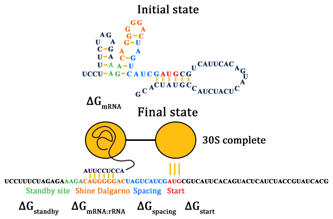
As for how to calculate ΔGtot, we need to know how the SD and ASD sequence compliment with each other. The Watson-Crick base pairs and G:U wobbles (red lines) are shown in Figure 3.
Given a specific mRNA sequence called the sub-sequence surrounding a start codon, ΔGtot is predicted according to an energy model (equation (3)), where the reference state is a fully unfolded sub-sequence with G=0.
In such ΔGmRNA:rRNA is the energy released when the last nine nucleotides (nt) of the E. coli 16S rRNA (3′-AUUCCUCCA-5′) hybridizes and co-folds to the mRNA sub-sequence (ΔGmRNA:rRNA< 0). Intramolecular folding within the mRNA is allowed. All possible hybridizations between the mRNA and 16S rRNA are considered to find the highest affinity 16S rRNA binding site. The binding site minimizes the sum of the hybridization free energy ΔGmRNA:rRNA and the penalty for nonoptimal spacing, ΔGspacing. Thus, the algorithm can identify the16S rRNA binding site regardless of its similarity to the consensus Shine-Dalgarno sequence.
ΔGstart is the energy released when the start codon hybridizes to the initiating tRNA anticodon loop (3′-UAC-5′).
ΔGstandby is the work required to unfold any secondary structures sequestering the standby site (ΔGstandby< 0) after the 30S complex assembly. We define the standby site as the four nucleotides upstream of the 16S rRNA binding site, which is its location in a previously studied mRNA.
To calculate ΔGmRNA:rRNA, ΔGstart ,ΔGspacing, ΔGstandby and ΔGmRNA, we use the NUPACK suite of algorithms with the Mfold 3.0 RNA energy parameters. These free energy calculations do not have any additional fitting or training parameters and explicitly depend on the mRNA sequence.
In addition, the free energy terms are not orthogonal; changing a single nucleotide can potentially affect multiple energy terms. The relationship between the spacing and the ΔGspacing was empirically determined by measuring the protein expression level driven by synthetic RBSs of varying spacing and fitting a quantitative model to this data.
Verification of the orthogonality
Since the two protein expression systems are orthogonal, the orthogonality should be one of the most important factors in our modeling. So the first important task of the dry lab is to predict the orthogonality.
If the two protein expression systems are orthogonal, the protein expressed through pathway 3 and 4 should be minute when compared with pathway 1 and 2. Therefore, we firstly calculate the individual protein expression level.
The individual ΔGtot is calculated according to the formula in previous section. Refer to the Calculation page for details.
| Pathway 1 | Pathway 2 | Pathway 3 | Pathway 4 |
|---|---|---|---|
| ΔGtot(kcal/mol) | ΔGtot(kcal/mol) | ΔGtot(kcal/mol) | ΔGtot(kcal/mol) |
| -4.7 | -6.28 | 3.73 | 4.93 |
According to the equation of protein expression level:
And under the hypothesis that the k, m, and Rtot remain the same in the four pathways because they happen in the same cell, we can arrive at the following results:
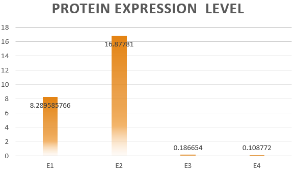
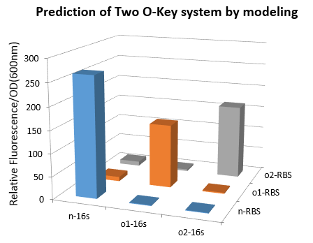
The results are shown in Figure 4. According to the results, we know that Pathway
E1 and E2 express considerable amount of protein, which indicates that the orthogonal system works just fine as works the canonical system. Furthermore, E3 and E4 is negligible compared to other two results. This show that the orthogonal ribosome cannot translate the canonical mRNA, and vice versa. Therefore, our system demonstrated great orthogonality, which goes very well with our experiment.
Modeling Based on Wet Lab and its Results
We have introduced ΔGtot as the indicator of mRNA-ribosome binding strength. Now, let’s take a look at the modeling and its relative ΔGtot.
We chose the red fluorescence protein (RFP) as the encoded protein of the n-mRNA, green fluorescence protein (GFP) of the o-mRNA. The final calculation results from the four pathways are listed below. For detailed calculation processes, please refer to the Calculation Page.
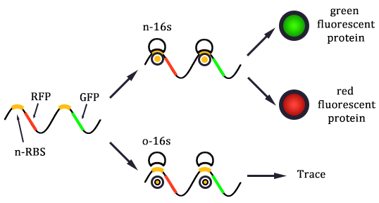
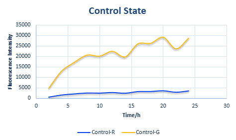
Before determine the amount of protein expressed, we established a control state (Figure 5).
Control State
In the control state, there are two proteins with normal RBS sequences and canonical ribosomes. The protein expression amount, as we have previously explained, is directly related to the binding ΔG of the first step.
The control state is the original state with only the canonical ribosomes and RBS, whose parameters can be obtained easily, whose data is also the foundation of our system.
The protein expression amount of the two protein at the control state can be expressed in the following two formula.
Experimental State ONE
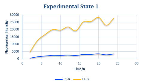
After the control state, we introduce the experimental state ONE. The design is shown in Figure 6.
In the experimental state ONE, the two genes have normal RBS sequence. But there are two kinds of ribosomes present: the canonical one and the orthogonal one. So we use x to represent the percentage of normal ribosome and y to represent the percentage of orthogonal ribosome.
The protein expression amount of the two protein at the experimental state ONE can be expressed in the following two formula.
In the formula, x and y means the percentage of normal and orthogonal ribosome.
Experimental State TWO
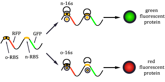
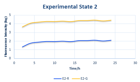
The design of experimental state TWOis shown in Figure 7.
The RBS sequence of GFP mRNA is normal, while that of RFP is orthogonal. As for the ribosomes, there are not only the canonical ones but also the orthogonal ones.
The protein expression amount of the two protein at the experimental state 2 can be expressed in the following two formula.
In order to eliminate the many unknown parameters, we use the relative expression amount to express. The result of relative expression amount are listed below and detailed calculation process are in the detailed Calculation Page.
Combined with the following wet lab data, we can calculate the exact value of x and y. What is more, we can also put x and y into the relative protein expression amount and to calculate the exact value of ratio. Combined with the curve of fluorescence varying with time in Control State obtained from wet lab, we can calculate the same curve of the two experimental state. Please refer to the following pictures.
Construction of Multi-Orthogonal Systems
After the design and construction of two orthogonal systems, the wet lab result verified the accuracy of the model. Then, we also created triple-orthogonal systems within bacteria. The prediction result is shown in Figure 12.
We can see from the figure that the protein expresion of diaganol line expression amount is significantly larger than that of others.
In the future we can also have the bold goals of the construction of multi-orhtoganol system theoritically feasible.
 "
"


