modeling
The ebb and flow of E. coli in computer..
1 Analysis of E.coli and Bdellovibrio’s growth in the number of speed by a group of photographs
Abstract: Based on the observations at intervals of several days, and the photos of the plaque in the process of E. coli and Bdellovibrio group’s growth in the same dish taken at a high resolution for experimental, we use of the image processing functions of Matlab to simplify the statistics and calculate the relative quantities of the two bacteria at the observation time in the dish. The results also verify whether the experimental results conform to the classical S-shaped curve, and estimate the bacterial growth rate in every moment, in order to analyze the bacterial growth’s features under the conditions of the experiments.
Key words: Bacterial growth High resolution photos Image processing S-shaped curve fitting.
1.1 The classical model of the flora growth
Under normal circumstances, a growth curve can be obtained with the time as abscissa and the logarithmic of the number of viable cells as ordinate. The curve shows the four periods of the bacterial growth and reproduction: the lag period, the logarithmic period, the stable period, the decline period. The lag period is the transient process the bacteria adapt to the new environment after being inoculated to the medium. In this period, the curve is flat and stable because of slow bacterial multiplication. The number of viable bacteria will soar when it reaches the logarithmic period. The bacteria will grow at stable geometric series, and can last sustainably hours and days (depending on the conditions and bacterial generation). Moreover, bacteria’s form, dyeing and biological activity in this period are all very typical which is sensitive to environmental factors, so it’s the best period to research the bacterial traits. When it reaches the stable period, however, the total number of flora is in the flat stages due to the relative relationship of nutrition and the number of bacteria, but bacterial viability changes greatly. Finally, bacterial growth will get slower in the decline period, and the number of the dead bacteria will apparently increase. In addition, the number of viable cells and the incubation time are in inversely proportional relationship. Mastering the bacterial growth’s law, we can study the method of controlling the growth of pathogenic bacteria, discovering and developing bacteria useful to human.
1.2 Assumptions and simplifications
1. Imagine that plaque is dense, that is to say, it’s always a simply connected area in surface of the two-dimensional dish.
2. Imagine that the plane occupied by the plaque in the culture dish is proportional to the number of bacteria in it.
3. Under the experimental conditions, imagine that E. coli is the only food of Bdellovibrio, and nutrients of E. coli are provided by the medium sufficiently.
4. The occasional small amount of bacteria in the edge of dish is ignored, and dripping or splashing a small amount of bacteria into the location of the error place in the initial state is considered to have no impact on the normal experimental bacteria.
5. After appropriate image processing, the light and its changes’ effects to the photos are ignored.
6. As to the fuzzy edge of the plaque, the area is considered to be the largest and smooth edges simply connected region.
1.3 Assumptions
3.1 Photos’ preprocessing
1. Select photos artificially. Remove the ones whose light effects apparently different from most of the photos, as well as the ones which appear the situation that two plaque overlap and stick together and the overlapping area is large in the later observations, so as not to increase the difficulties of unified image processing.
2. Rename all the photos by unified format. The format is ‘experimental group + days + hours + minutes xxx’, (such as ‘3111111’ meaning the third group at 11:11 on the 11th), which is beneficial to the unified automatic processing.
3. The few overlapping points of two plaques are considered to have no effects on these two, so use Photoshop to change the connections as the background color, in order to processing uniformly.
3.2 Calculation of the plaques’ area
1. After reading the photos, select the appropriate threshold to transform the photos into a binary image, according to the light conditions.
2. Identify all the connected regions, and remove the smaller ones (maybe caused by useless bacteria or lens’ dust).
3. Because of the light and its reflection in every photo, the edges of culture dishes are always lit, which require removing the large connective regions in the edges.
4. Calculate the area of the other connective regions, which is all the plaque area.
5. Use the area above as the relative number of bacteria, and pixel as the unit. Similarly, the number of bacteria growth rate is in unit of pixel/ unit time. And it is the same way if ‘the number of bacteria’, ‘the relative quantities of the bacteria’ and ‘the rate of bacteria growth’ in the paper is not particularly described.
1.4 Results and analysis
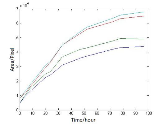
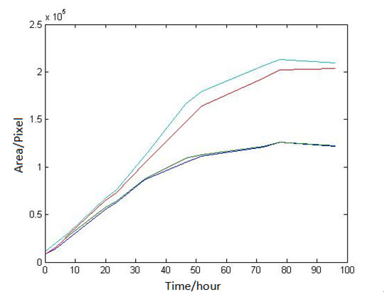
4.1 Figure of the changes in the number of E. coli and Bdellovibrio
Fig 4.1 Changes in the relative number of E. coli
Fig 4.2 Changes in the relative number of Bdellovibrio
Specific statistics can be seen in Appendix.
4.2 Changes in the number of experimental bacteria and comparison with the classic model
The method of judging whether the image processing above is reliable is to verify whether the number of bacteria conform to the S-curve changes over time. Furthermore, it is to select some appropriate forms of S-shaped curve and if the fitting results is relatively good, the data are regarded to be consistent with the S-shaped curve, that is to say, the image processing method is credible.
Select the logistic function used to describe the symmetric S-shaped curve to fit. The expression of the logistic function is:
(4-1)
Where A,B,C are unknown parameters.
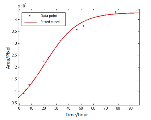
Use ‘cftool’ in Matlab to fit the eight groups of data of the eight plaques, with the default method of least squares. After selecting the appropriate initial value for the three parameters, the results can be obtained quickly. By the fitting of eight groups of data, we found all the right parameters A,B,C to make data points distributing on both sides of the fitted curve and variance is small. If so, it is considered that the eight groups of data conform to the S-shaped curve, and that the image processing above is reliable
The fitting results of a particular group are as follows:
Fig 4.3 Fitting results of S-type curve
Fig 4.4 Fitting results analysis in Matlab
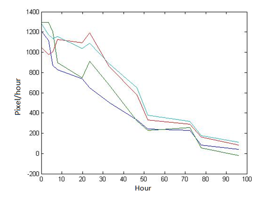
4.3 Estimation and analysis of the rate of experimental bacteria growth
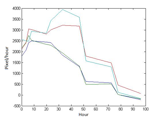
Fig 4.5 Growth rate of E. coli
Fig 4.6 Growth rate of the Bdellovibrio
Specific statistics can be seen in Appendix.
The method of calculating the growth rate here is to calculate the difference quotient.
It is shown in the figure that there are all downward trends in the growth rate of E. coli and Bdellovibrio. The growth rate rebound in the 30th to 40th hour, which is likely to be affected by the large base of bacteria and the rich surrounding nutrients. In addition, the rebound of E. coli within 20th to 30th hour may be influenced by changes in light intensity in the fourth, five photos( respectively shooting at 19.8 and 23.5 hours).
If the plaque is regarded as a single connected area with smooth edge, the radius of curvature of a point can be obtained by the image processing, so the outwardly extending rate in the radius direction at a certain time can also be obtained by solving a quadratic equation.
1.5 Shortcomings and improvements
1. Since the first step of the image processing requires threshold value pictures, therefore the lighting situation, especially in light colors and light intensity, have a significant effect on the results. Accidental illumination changes caused by tiny accidental error can be ignored, but it must be required that the natural light is weak, and the indoor light, camera distance, angle and camera parameters must remain constant at least in the same set of photos, in order to avoid systematic errors. However, we did not notice in the experiments when taking photos, so that the light intensity of the first to the fourth sheets of the third group is significantly different from the ones after the fourth photo. Even though the appropriate processing is performed by changing the binarization threshold, there inevitably exist some small systematic error. If the similar phenomenon can be avoided in the next experiments, the accuracy of the data will surely be able to improve.
2. In the 6th assumption, ‘As to the fuzzy edge of the plaque, the area is considered to be the largest and smooth edges simply connected region. ’, which really brings convenience to the image processing, but it will make a large systematic error in the calculation of the number of bacteria produce. Taking into account that the experimental purpose is to explore the elongation ability of the bacteria in the unit time in the dish plane, however, and the main aim of the calculation and analysis of the number of bacteria is to increase the reliability of classic model. Therefore, this error can be accepted.
3. Plaque on a plane may be different in thickness; there may be impurities in plaque; plaque may also be non-dense. The factors above will all result in the absolute number of bacteria is not proportional to the area of plaque on the photo. If the error cannot be ignored, the calculation of the number of bacteria will be influenced. But as it is described in 2, they do not affect the primary purpose of the study.
1.6 Reference
[1] 许金泉,张娟,马琼瑜,李云.细菌(数量)生长规律的数学模型[J].云南大学学报(自然科学版),2008,30(S2):157~159.
[2] 夏结来,徐雷,陈长生.S型曲线的一种新的拟合方法[J].中国卫生统计.2001,18(4),195~197.
1.7 Download
You may download pdf. version of this article here:
Analysis of E.coli and Bdellovibrio’s growth in the number of speed by a group of photographs. pdf
2 A Spatial Model of Plasmid Conjugation Transfer on an Agar Surface
2.1 Summary
There are two main kinds of scheme to do the bacterial plasmid conjugation experiment: in well-mixed solution, or on solid culture such as agar surface. To spread the ‘death gene’ better in our ‘toxic apple’ project, we want to do some research on how to improve the conjugation efficiency under certain conditions. IGEM_Berkeley Team of IGEM 2005 have done some experiment on conjugation in solution and gave the best ratio between initial D(donor cells, similarly hereafter) and R(recipient cells) as 1:2. However, aimed to improve the conjugation efficiency, we consider the experiment and analysis of conjugation in solution are with these disadvantages:
1. The process of the experiment is difficult to be seen by an electron microscope.
2. The result is random in a certain degree due to the large space that cells could freely move in and the complex dynamics system of cells in the solution.
3. Mixing the solution is a necessary step to help D and R contact while it may also interrupt the conjugation itself.
Taking the reasons above into consideration, we decided to model for the scheme on solid culture. Due to the limited time in our experiment, we use some parameters from others’ experiment and modeling and we also use the SDTC model to get the best ratio between initial D and R with the total number of initial plasmid donor cells and recipient cells constant by simulation.
In our SDTC model, we employ a lattice of 500×500 to describe each cell and each sites in simulation lattice area separately so we can trace their state separately at any time. We use a ‘Cycle Time Trace’ system to record each cell’s doubling and conjugation state and ensure they update asynchronously so that the time in our system could be considered as continuous compared with the scale of cell doubling time or conjugation cycle time though any kind of simulation of time has to use a small period of time as simulation step length and we make no exception.
2.2 Model
2.1 Space system
In the SDTC Model, we set up a 500×500 lattice which contain 250000 sites. Bacteria and nutriment can be at any site on the lattice. The bacteria cell is considered 1 um2 that the total area of our view window is 0.25mm2.
Furthermore, the lattice can be extended to more than 2 dimension. The thickness of lattice has three possible value: 0, 1, 2, that is to say, each site can hold mostly two kind of bacteria at the same time. In addition, there is no such ‘up and down’difference inside one site in this 2.5D model. The thickness of nutriment is 0. The reasons why we set this model like this are as follows:
1. The model abstracts the thickness of bacteria into three levels, making the modeling and simulation able to be built and operated in several lattices, which greatly reduces the difficulty of modeling and the time of simulation.
2. Some three-dimensional properties are added to the SDTC model. For example, the filial generation comes out randomly around the parental generation. If the two layers of the neighborhood were taken over, the division will however be controlled. In a word, the SDTC model is a 2.5D model.
3. The model also largely simplifies the judgment of donor cell and receptor cell in conjugation (the conjugation occurs only when the donor cell and receptor cell are at the same site).
We introduce the conception of ‘neighborhood’ in our plane domain and divide it into ‘bacteria neighborhood’ and ‘nutriment neighborhood’. As to any point, the bacteria of the bacterial neighborhood mean all the bacteria in the center of the 3 × 3 square area; similarly, the nutrition of the nutrient neighborhood refers to the nutrient in the center of the 7 × 7 square area. The detailed reasons of setting like this were discussed in Reference [2].
It is considered that bacteria can reproduce and transfer only within a certain distance due to the use of agar medium, but bacteria and nutrients cannot move. This is the fundamental difference between this model and the model in solution.
2.2 Bacterial and nutrient system
E. coli can be divided into three categories: D-donor, R-receptor, T-conjugative transfer receptor. Considering the bacterial horizontal conjugative transformation and reproduction, their speeds are related to the quantity of nutrients in the neighborhood, which is conformed to the beta function (a sigmoidal function). Specifically, there are two thresholds - the lower one C1 and the upper one C2. When the quantity of nutrients in the neighborhood C
C1, reproduction and conjugative transformation will do at a highest speed Ψ2 and γ2 respectively. Ψ2 of the three bacteria D, R and T are different. When C2>C>C1, the speed of reproduction γ and the speed of conjugative transformation Ψ obey the distribution of C Linear within the minimum and maximum.
In the condition that there are nutrients in the nutritional neighborhood, D and R that are at the same site on the layers of different thicknesses begin conjugative transformation, while the division process always exists.
The repression has always been difficult in the modeling of conjugation. Most of the F plasmid is with repression. In our SDTC model, we deal the repression as the balance between the conjugation and division, or between the horizontal and vertical plasmid transfer . By introducing a penalty factor p and using our cycle time trace system, we are able to describe this balance. Once a bacterium experience one type of plasmid transfer(horizontal or vertical), another type’s cycle state of the site (which recorded by cycle time trace system) clear, as another type of plasmid transfer need to restart the preparation of energy and the bacterium itself. Besides, the cycle length of the second one change to p times of standard length ,which means the other kind of transfer need more preparation time.
We introduce a random factor τ to describe the plasmid loss. When D or T begins to split and multiply, their filial generation has the probability of τ lose the plasmid and become an R.
The filial generation that bacteria reproduce disperses randomly in the center of the 3 × 3 square area including them. But the offspring may ‘die in the womb’ when the number of bacteria around its site reaches the upper threshold due to the limited space in the medium.
Because of the use of agar medium, if the nutrient at a certain point is consumed, it is completely consumed and will not regenerate, nor be replenished by the surroundings.
Each reproduction consumes the nutrients in the nutrients neighborhood. If the nutrients in the neighborhood exhaust, the bacteria cannot reproduce. More precisely, they will firstly choose which distance-level of neighborhood nutrients to take in according to the proportion of the bacterial number and distance in the certain level(closer level has better chance), then, in the chosen level, which nutrient to choose will be determined by the random selection in direction. This algorithm has some advantages as follows:
1. The closer nutrients are more likely to be consumed.
2. Isotropic of nutrient consumption can be maintained.
3. The algorithm is simple.
2.3 Cycle time trace system
Set 40min as the standard time which receptor cell breed a generation take, which is to say Ψ2 (R) =1.0. Ψ2 (D), Ψ2 (T), γ2 are all the relative value to Ψ2 (R). The rate of division and conjugation of bacteria at each point is decided by the quantity of nutriment in the neighborhood, making the update time of each point different. The details are as follows:
1.Initialize three cycles of tracking plane the same size as the simulation plane.
2.Two planes of two layers record the progress of bacteria's division cycle. Where there is no bacterium at the point of the plane, the progress of it is constant 0 .The third plane records the progress of conjugation cycle. The progress is not 0 only when there is a D and an R on the same site at the same time.
3.All the three planes need to be calculated at each step of the simulation. With the time of each simulation setted L minutes and r employed as the relative division rate or relative conjugation rate at that point of the plane. r×L/40+ξ will be added to each step and point according to rule 2, where ξ is a random factor. If the value of a certain point reaches or gets larger than 1 after a simulation, the value subtracts 1 and note the split /conjugation occurs once.
The advantage of this cycle time trace system is:
1.Being able to trace and record the progress of the division and conjugation at each point and plane in the cycle and make it convenient to improve SDTC to more complex models later.
2.SDTC model time can be considered as continuous. Because of the different relative division and conjugation rate of different cell, the update of each point on plane is asynchronous. Actually, any simulation that operates with the time has to set a small step size. Once the step is tiny enough and the elements’ update is asynchronous, we can say the time is continous.
3.Easy to deal with the program and simulation.
2.4 Initial state
D and R are randomly distributed of certain density in the two layer planes. The density of each plane can be controlled respectively. The nutriment filled the whole plane uniformly.
2.3 Assumptions
We use The SDCT model established above to simulate within the observation area of a lattice with its side length setted 500. Di (R) + Di (D) = n (Di (X) is the initial density, n is a predetermined value). We want to figure out the relationship of the ratio between Di (R) and Di (D) and final density D(T). .
We have the following description with the setting:
1.As the total number of the nutrition in the square region is limited, and competition occurs among conjugative transfer and reproduction nutrient. too high or too low initial density both cause conjugative transfer fewer. Therefore the initial density and must be limited within a certain value range.
2.Due to reproduction and conjugative transfer both breeding competition on nutrition, and we need to study the the ratio of D and R conjugative transfer efficiency, we should control the reproduction competitiveness, so then initial density is set to a fixed value.
3.the ratio of the optimum D and R may vary within a certain range with n. Here only consider one value of n.
The simulation results are shown as below:
Wherein C2 = 4, C1 = 1, γ1 = 0, γ2 = 6, Ψ2 (R) = 1.0, Ψ2 (D) = Ψ2 (T) = 0.9, τ = 0.005, p = 1.0,
n = 0.08.
Simulation step length is 1min. The maximum time limit of simulation is 30 hours. The simulation should be terminated when the total number of plane nutrition is less than the initial value multiplies 0.001.
As is shown in the picture, the best ratio of D and R is 3:2. The simulation is terminated as nutrients running out. The final state of the two layers of bacteria are shown below:
2.4 Shortcomings and improvements
1. Because of the limitation of experiment period and condition, some parameters in our simulation come from others’ model and experiment. Since the experiment conditions are different, the parameters may be impertinent. We can calculate every parameter more carefully and improve the accuracy of model if we have more time and resources.
2. The model and simulation of the repression of conjugation has always been the difficulty of conjugation models, thus rarely can we find the related reference model and experiment. Set out with the conception of balance each other, we come up with a model of two plasmid transfer types which one can inhibit another one. But the correctness of this model still need more experiment to be testified.
3. Due to the limitation of condition, large-scale computers are not available. We could have set a smaller simulation step length or improve the accuracy of simulation to acquire a better result.
2.5 References
[1] Simonsen. Dynamics of plasmid transfer on surfaces [J]. Gen Microbiol, 1990, 136: 1001–1007.
[2] Stephen M. Krone, Ruinan Lu, Randal Fox,Haruo Suzuki and Eva M. Top. Modeling the spatial dynamics of plasmid transfer and persistence [J]. Microbiology, 2007, 153: 2803–2816.
[3] Zhou Hongjin, Wang Xiusen. Massive Data Process Methods Based on Matlab [J]. Computer & Digital Engineering, 2012, 271: 89-90, 103.
[4]IGEM_Berkeley Team of IGEM-2005. Part: BBa_J01003: Experience[EB/OL]. http://partsregistry.org/Part:BBa_J01003:Experience, 2005-10-18
2.6 DownloadReferences
You may download pdf. version of this article here: The SDTC Model (iGEM 2012 SEU A Model).pdf
Copyright © Southeast University iGEM 2012 Team A, All rights reserved.

 "
"

