"

From 2012.igem.org

Contents 1 Modeling Bacteria 1.1 Are you hungry? 1.2 Are you hot? 2 Modeling Yeast

Modeling Bacteria

Here we modeled several of the Bacteria constructions.

Are you hungry?

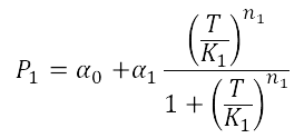
The first models we did is for our glucose-sensitive construction. We carried out three different experiments changing the carbon source, to see its influence. First we used glucose (1) as the only carbon source, then we added galactose (2) as an extra carbon source and then we put sodium acetate (3) as an extra carbon source instead of galactose. This is because we checked in previous tests that low concentrations of glucose compromised cell growth. With the experimental data we fit the following repressible hill function.

And we estimated the following parameters for the 3 different conditions.

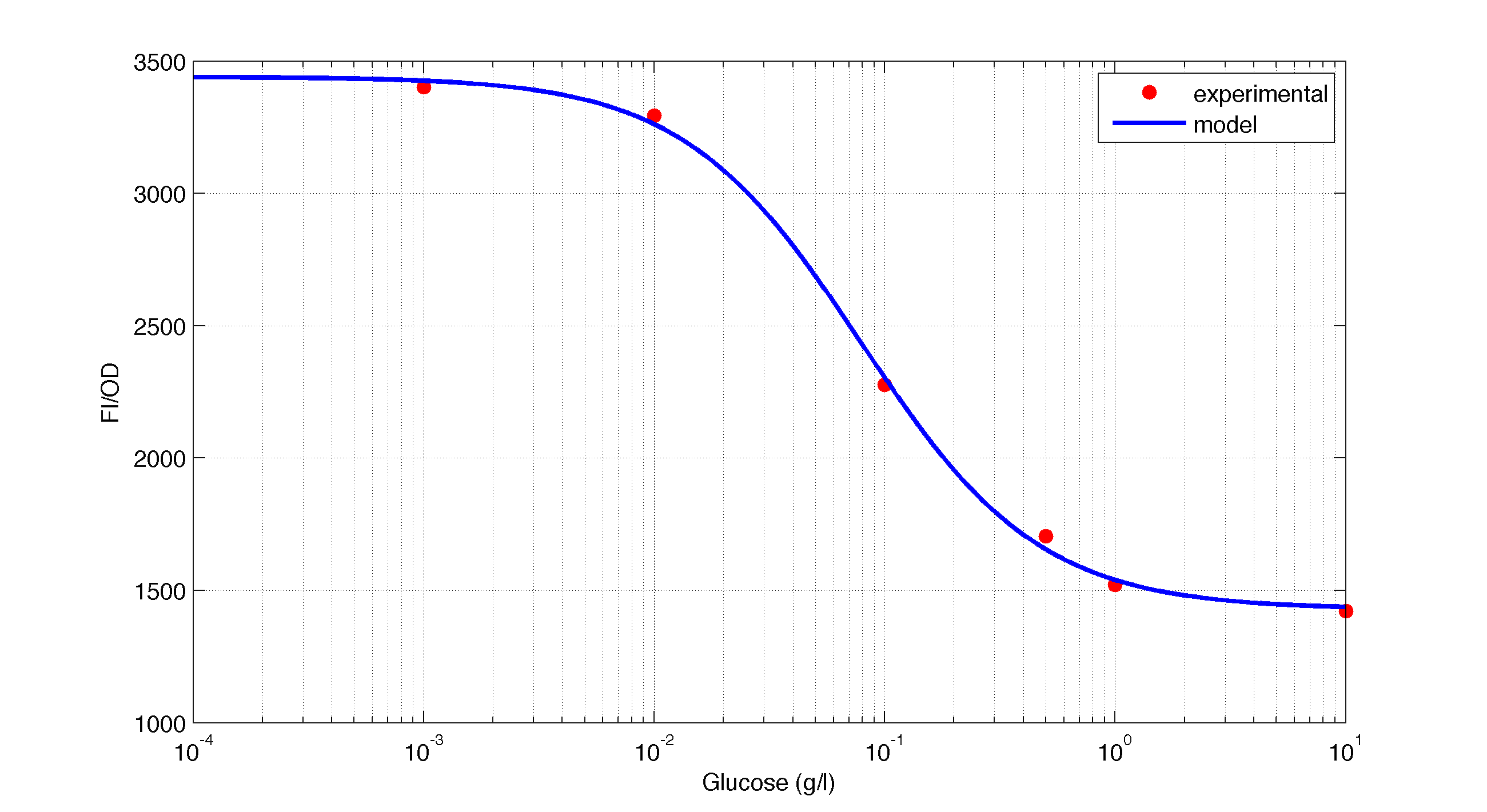
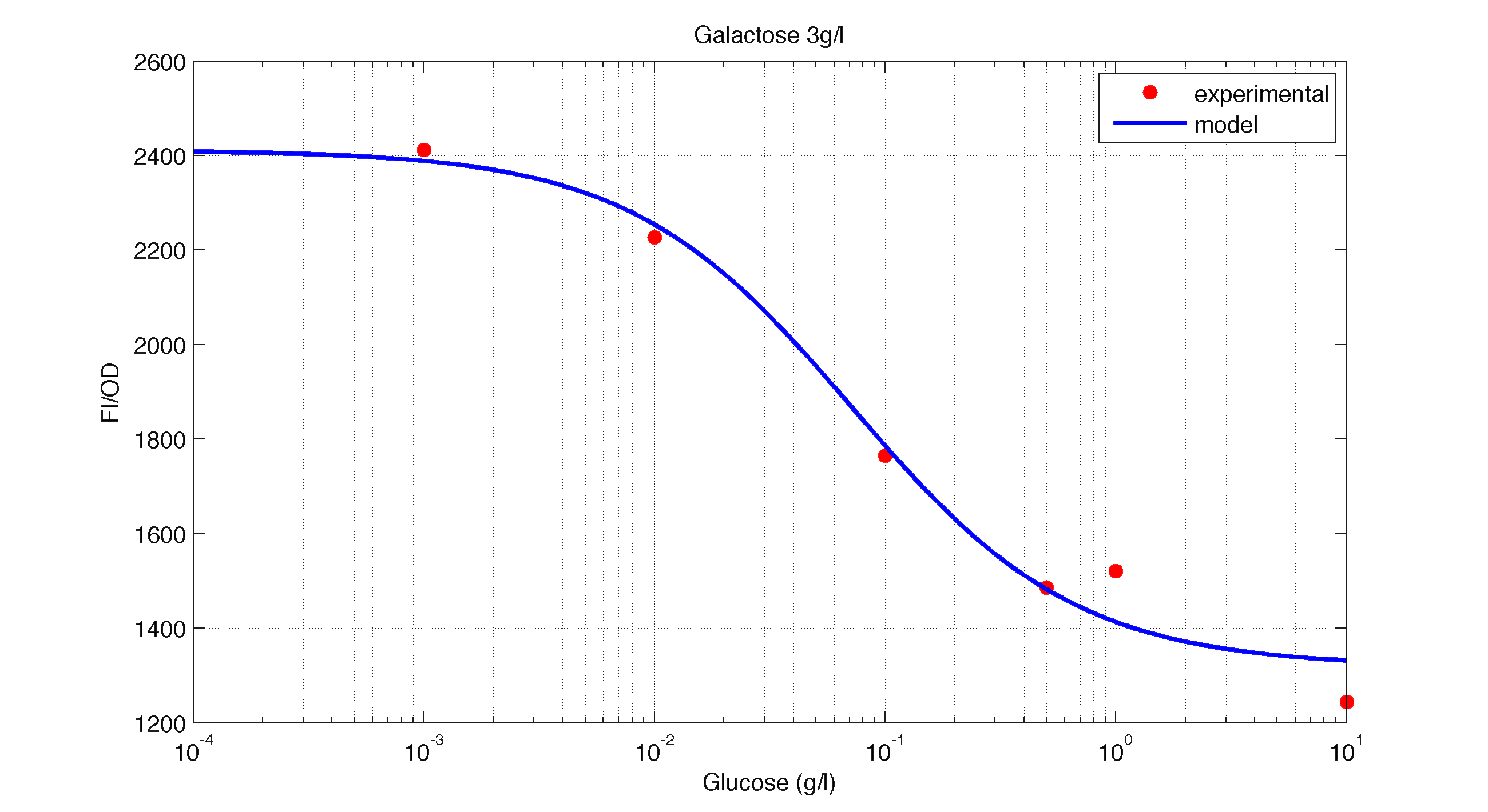
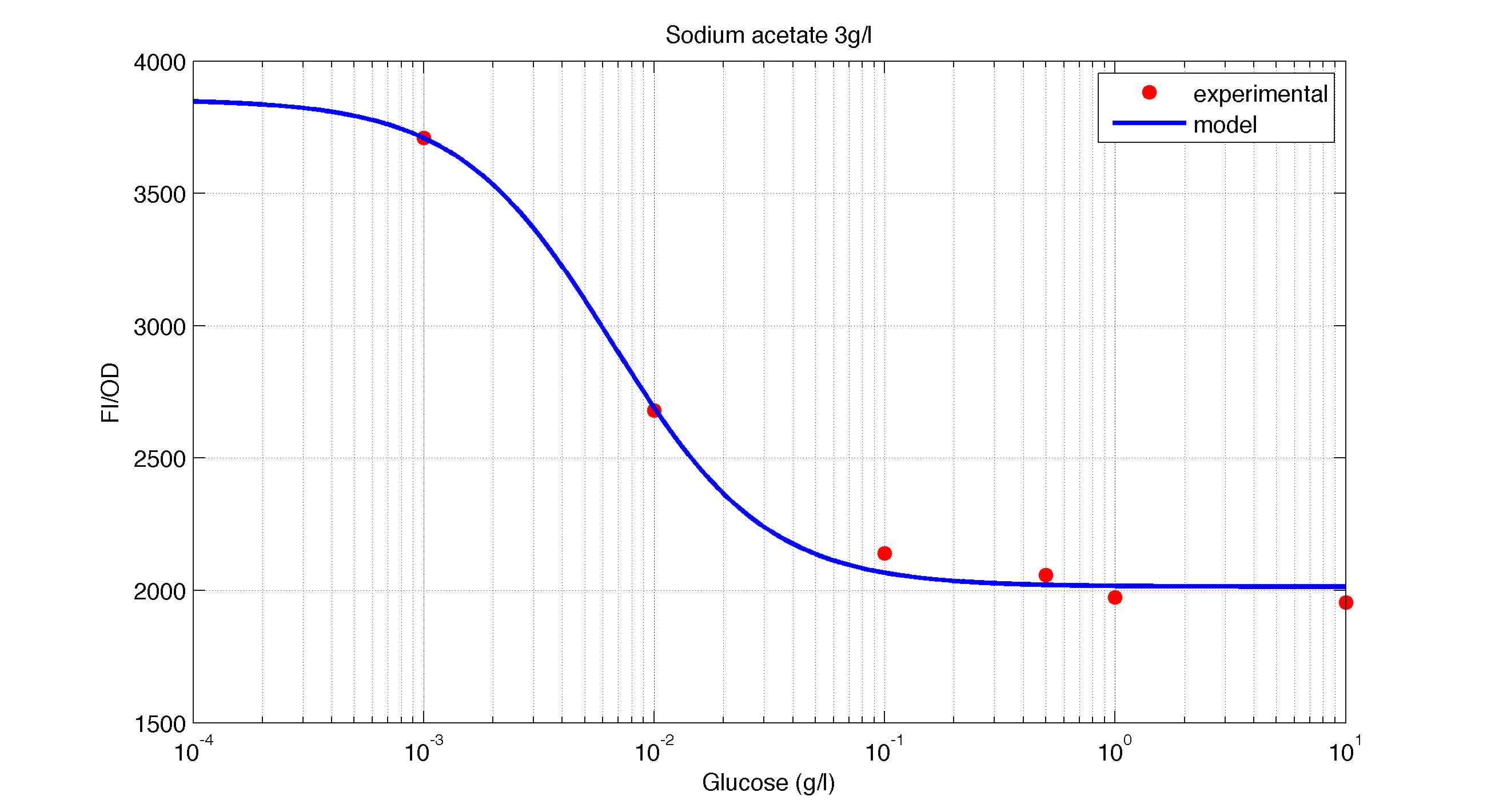
In figures 1, 2 and 3 we plot the models and experimental data for the three experiment with glucose (1), added galactose (2) and added sodium acetate (3) respectively. IPTG was added to all the experiments to induce expression.

Figure 1. Model and experimental data for different glucose concentrations.

Figure 2. Model and experimental data for different glucose concentrations with 3 g/l of Galactose added to the medium.

Figure 3. Model and experimental data for different glucose concentrations with 3 g/l of Sodium Acetatee added to the medium.

Are you hot?

For the case of the Heat Shock promoter, we decided to model the static transfer function of the Fluorescent Intensity as a result of the Temperature with the following equation:

In order to estimate the parameters of this model we performed a heat shock experiment.

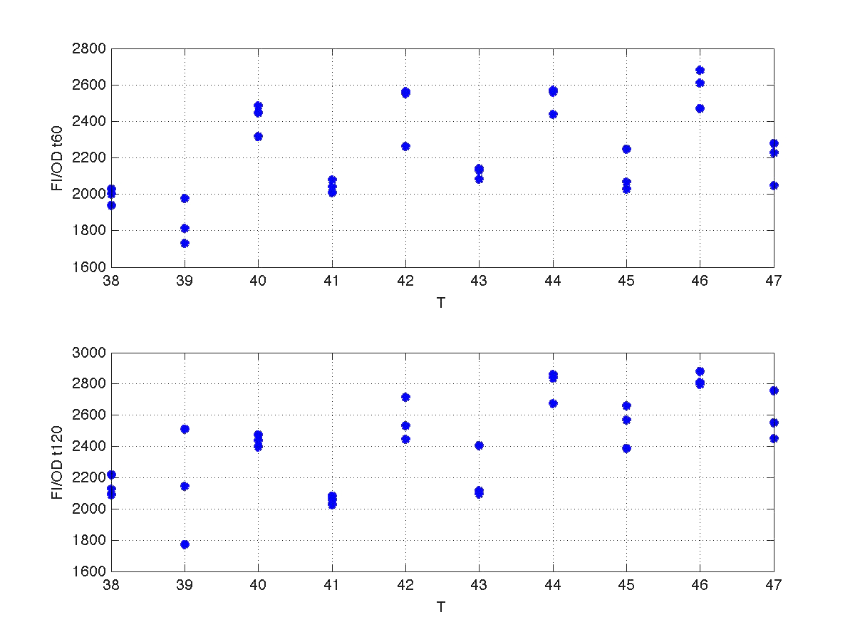
Analysis corresponding to a heat shock applied during 10 minutes at different temperatures ranging from 20ºC up to 51ºC. For each temperature three samples were tested. Fluorescence Intensity (FI) and optical density (OD) were measured at t1=60 minutes and t2=120 minutes after application of the heat pulse had finished.

The first practical problem we encountered was the lack of enough heating coats. Because of these we took the culture, and we splitted the experiments in two batches. FI and OD were measured at t1=60, and t2=120 for batch number 1, while for batch number 2 the heat shock was delayed by 40 minutes with respect to the first batch. Therefore, measu-rements for batch no.2 were taken at t1=100, and t2=160 minutes respectively.

During this 40 minutes delay, the microorganism was growing. Therefore, the heat shock in batch no. 2 was applied to a larger population than in the case of batch no.1. Consequently, the measurements of FI and DO gave much higher values. This affects the ratio FI/DO, were the two batches can be clearly distinguished (see figure 4).

Figure 4. Raw data from the heat shock experiment.

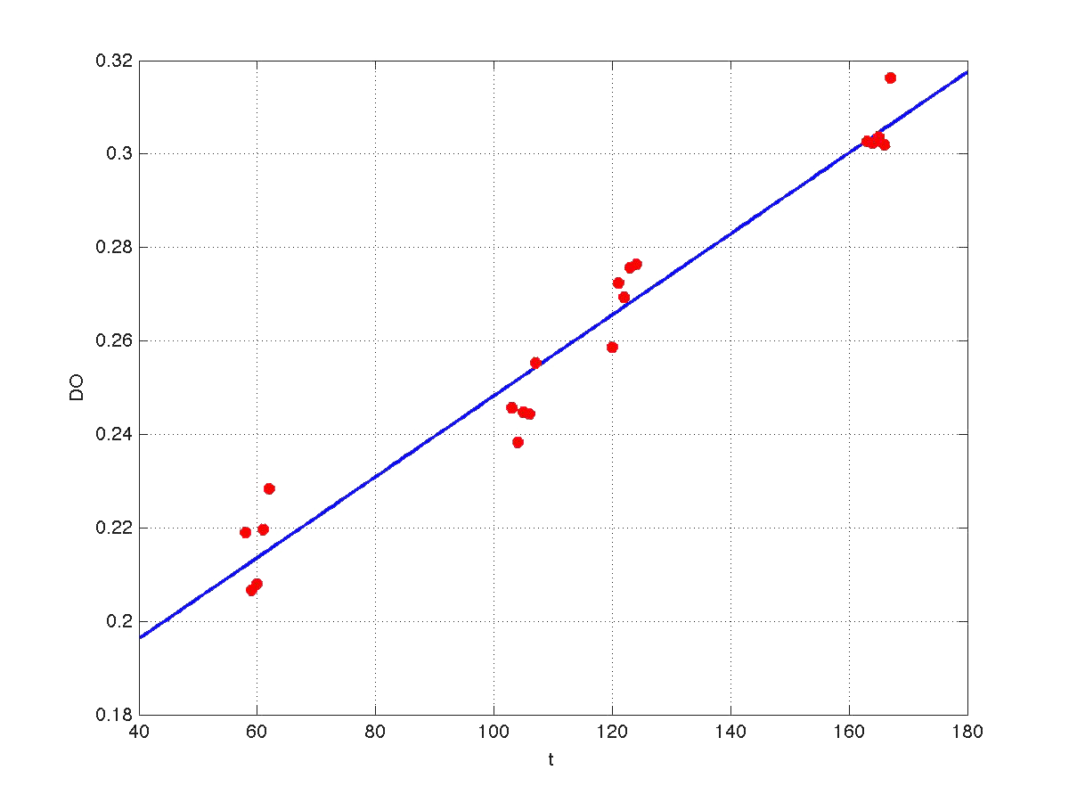
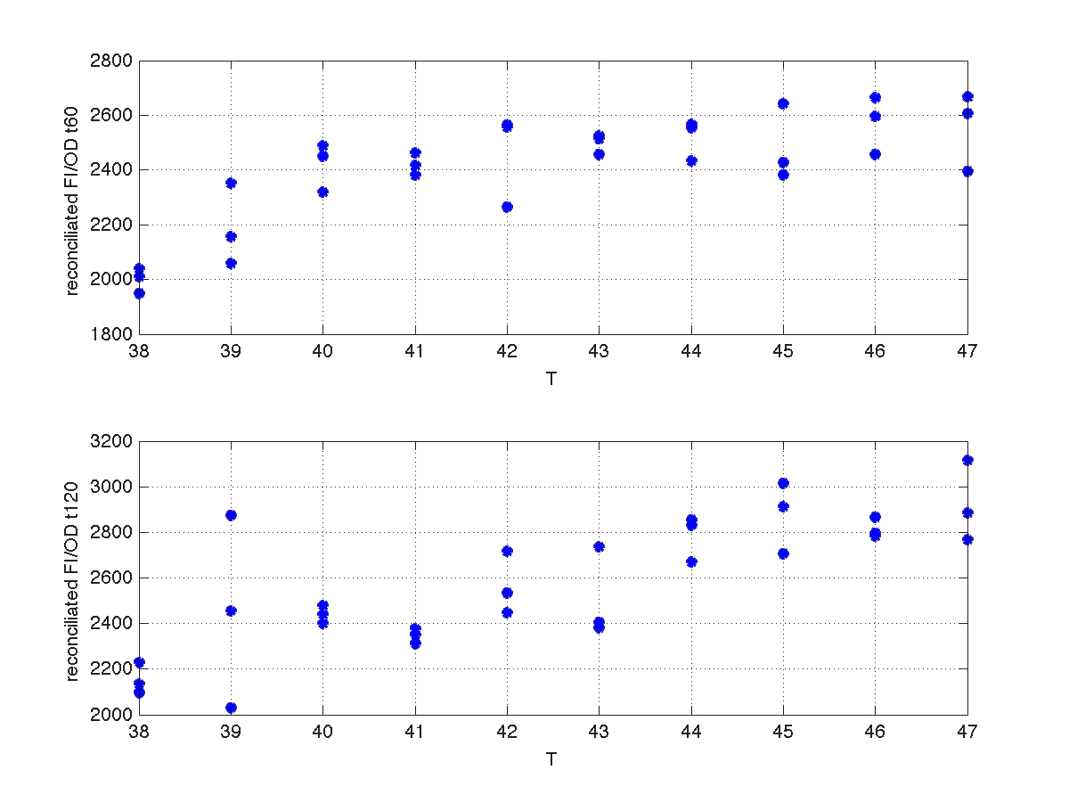
Our first modeling work was to perform data reconciliation. To this end, we assume that during this 40 minutes delay the only thing that happended was that cells grew. Growth was approximately linear in the range analyzed, as seen in figure 1 (blue data). We fitted a simple model DO=p1+p2*t. The result can be seen in figure 5, were: p1 = 0.161573 p2 = 0.000866314 Therefore, the ratio FI/DO above can be compensated by multiplying data by the frac-tions (p1+p2*t100)/(p1+p2*t), and (p1+p2*t160)/(p1+p2*t). Actually, what we did was to compensate all measurements to the same time base. The reconcialited result can be seen in figure 6.

Figure 5. Model fitting for OD w.r.t. time.

Figure 6. Recoinciliated data for t=60min and t=120mins.

Once we had all data reconciliated we fitted it to a static model relating the ratio be-ween fluorescence intensity (FI), and the culture optical density (OD) with the temperature applied during the heat shock.

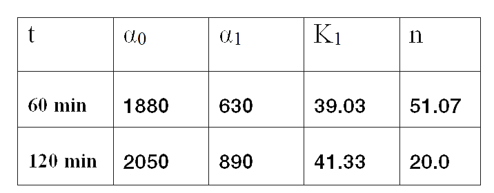
Since the model is nonlinear with respect to parameters K₁, and n, we applied a global op-timization algorithm based on stochastic search. Actually we applied it to fit the data at t=60 minutes, and t=120 minutes independently. The estimated parameters were:

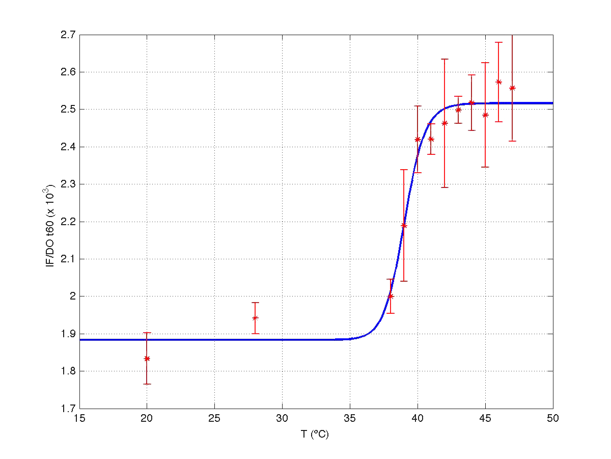
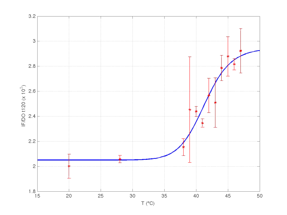
The results can be seen in figures 7 (t60), and 8 (t120) respectively.

Figure 7. Model and experimental data for t=60min.

Figure 8. Model and experimental data for t=120min.

Compare this results with Are you hot? results.

One question of interes is whether the increment observed in the ratio IF/OD is caused by an incement of fluorescence during the time elapsed, or it is caused by a varying dilution effect due to a decrease in the specific groth rate during that period [1].

To answer this question notice that the absolute growth rate can be obtained from the regression model OD(t)= p1+p2*t obtained above. Notice t is expressed in minutes in our model. Indeed, the specific growth rate at time instant t can be roughly estimated as mu(t)= [dOD(t)/dt]/OD(t). This gives mu(t) = p2*60/(p1+p2*t) if mu(t) expressed in h^(-1).

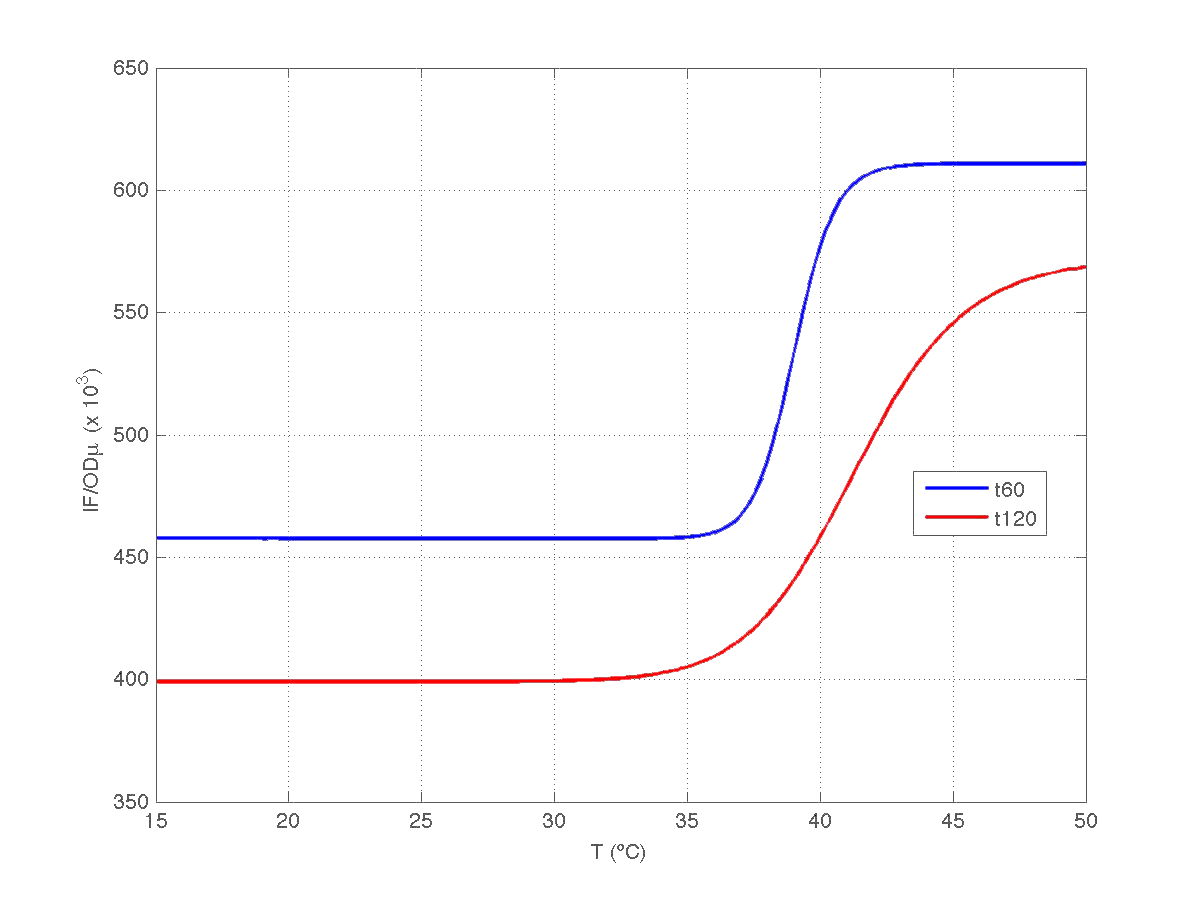
Therefore, we took our models and weighted them by mu(t60) and mu(t120) respectively. The result can be seen in figure 6. Indeed, the increment observed in fluorescence from t=60 to t=120 minutes could have been caused by a dillution effect. Of course, the main point to keep is that the ratio IF/OD (or, alternatively IF/OD*mu(t)) increases with temperature. So...our construction works!

Figure 9. Model IF/OD*mu(t) w.r.t. temperature for t=60min, and t=120min.

[1] S. Klumpp, Z. Zhang, T. Hwa, Growth Rate-Dependent Global Effects on Gene Expression in Bacteria, Cell 139, 1366-1375, 2009

Modeling Yeast

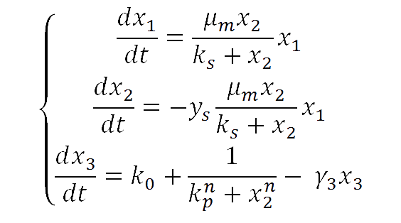
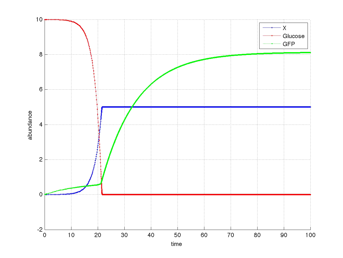
For our yeast construct: How long have you been fermenting? we propose a phenomenological model to explain the relationship between glucose concentration and fluorescent protein production. The following model was assumed:

where

x₁ = concentration of yeast
x₂ = concentration of glucose
x₃ = fluorescent protein
γ₃ = degradation/dilution rate for the fluorescent protein
k₀ = basal production of fluorescent protein
k_pⁿ = Hill-like coefficient. Notice the exponent n that also appears associated to x₂.

The graph below shows a simulated theoretical time evolution for the three variables.

As observed in the figure, once the glucose is depleted, the concentration of fluorescent protein increases from a basal value. Compare this results with Yeast fluorescence results