Team:Colombia/Modeling/Stochastic

From 2012.igem.org

Template:Https://2012.igem.org/User:Tabima

Stochastic Model

The previous sections showed how to know the mean behavior of the system for one cell, but this is just an average of the total proteins within the cell. All the biological systems are controlled by probability events. The cell is a huge space where there are a lot of small molecules, if we want a biological process to happen, two of this little molecules have to find themselves between million of other molecules in a huge pool. Also there is a possibility that a cell may need more concentration of a promoter’s activator while other may need less if the day is sunny but if is cloudy the second cell may need more. The differential equations don’t take into account these uncontrollable events that can change the response dramatically.

If we look only one cell, with all the uncontrollable events this may not behave like we want and the system may not respond or even worse the probability of dying exist and our cell may die. But dealing with one cell is not real, we always work with hundreds of cells. Within this population some cells may no produce the expected response but the others will and the average of cells would be able to respond to the presence of the pest.

The stochastic algorithms are a way to model these probability events within a population. This simulation are made in order to confirm that the system dynamics are robust and consistent and show us if the response is still behaving like we want after taking probabilities considerations. We use the Gillispie method to develop our model. Here is a brief explanation of how it works:

The complete method consists of eight steps.

1. Define the number of cells.
2. Define the time of the simulation
3. Define and name all the constants involved.
4. Define creation and destruction expression for each substance involved: The differential equations in this part have to be divided in two, the creation and the destruction expression.
5. Apply Gilliespie algorithm:
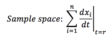
   1. Calculate the sample space of the analysed system: This is the sum of all the changes presented at specific time t.
      
   2. Calculate time distribution that depends on a random number between 0 and 1.
      
   3. The Gillespie algorithm does not consider simultaneous events, it says that each time only one event occurs. In our case the events are the creation or destruction of one protein. Each event has a probability of of occurrence within the sample space between 0 and 1. To know which event occurs at the time t+1 we take into account the random number use for the time distribution and look for the event that has this probability of occurrence . For example if you see the sample space figure below, there are 5 possibles events with their probability; if the random number is 0.4 then A is gonna be destructed but if the random number is 0.55 then B will be created.
      
6. Take the outputs from the simulation and convert them into regular interval vectors.
7. Obtain the Gilliespie function mean values.
8. Plot the obtained functions.