"

From 2012.igem.org

Companel|DNA calculating competitive reactions

During the course of our project we encountered a question that we had never before thought about. We were thinking about different ways to synthesize a TAL protein. One of the ideas was to take advantage of the thermodynamic behavior of different DNA strands and synthesize a TAL proteins by means of different primers that anneal at different temperatures to the template strand. We thought it to be possible to elongate a sequence by using this mechanism - simply changing the annealing temperature slightly whilst running a usual PCR. We assumed that the difference in optimal annealing temperatures of different primer sequences would favor one replication product over the others. The only thing we did not know was if this was significant enough to be used for the assembly of at least ten TAL domains. After unproductive research on this issue we decided to try modeling this scenario ourselves. The result of these efforts is CompanelDNA, an excel application that allows for predicting the equilibrium concentrations of competitive annealing. It can of course be used for every kind of chemical equilibrium where two substances compete for reacting with the same third reactant.

Theoretical background

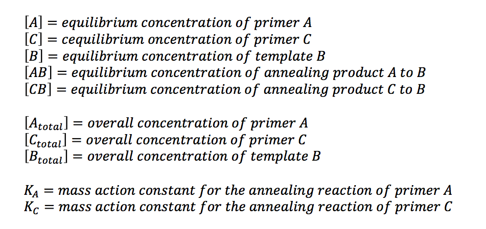
Although it seems to be a simple scenario, we did not find any preexisting solution to this problem - which came to us as quite a surprise. So we started by looking at the law of mass action behind the annealing reaction. Hereafter we shall use the following abbreviations and symbols:

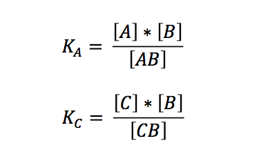
The laws of mass action for the two independent reactions are:

If we want to know what is going to happen to the concentrations we originally put in our reaction/PCR tube, we can expressed the term in relation to the overall concentrations:

Bearing in mind that the only unknown variables are (AB) and (CB) (K can be calculated, see below), one would try to solve these two equations with two variables. A number of other equations can furthermore be generated. However, these equations had no exact solutions when we used Mathematica to have them solved. All the proposed solutions are not applicable to a wider combination of parameters. Even when we asked for mathematical advice (thanks to Paul Staab, Munich) we got no further. So we decided to solve graphically instead (thanks to Konrad Schieban, Zurich). In order to do so the equations need to be solved for one variabel:

These equations can now separately be calculated by varying the variable (AB). When a value of (AB) is found that yields the same value of (CB) in both equations, both conditions are fulfilled. Graphically this would be represented by the intersection of the graphs of both equations. Basically this is what our application does.