Team:British Columbia/Consortia
From 2012.igem.org
(→Equations and Constants) |
(→Equations and Constants) |
||
| Line 31: | Line 31: | ||
| - | In the above equations, some of the key constants for the Monod Kinetics are obtained through analyzing the growth curves in a 96-well plate | + | In the above equations, some of the key constants for the Monod Kinetics are obtained through analyzing the growth curves in a 96-well plate, with varying amino acid concentrations. Characteristic growth rates were observed and plotted: |
[[file: GrowthRatesAA_university_of_british_columbia.png|center|700px]] | [[file: GrowthRatesAA_university_of_british_columbia.png|center|700px]] | ||
Revision as of 19:07, 3 October 2012

Modeling Microbial Consortia: The Auxotroph Approach
https://static.igem.org/mediawiki/2012/1/1f/Model_animation.swf
To gain a predictive understanding of consortium dynamics in the wet lab, we chose to model a system of simple auxotrophic interdependence. This system also enables us to establish a rapid foundation for which to conduct preliminary model refinements.
The three interdependent E. coli auxotrophs studied in our project are ΔtrpA, ΔmetA, and ΔtyrA. These three strains are deficient in the production of the amino acids tryptophan, methionine, and tyrosine, respectively. Thus, in order for each strain to survive, they must exist in the context of a consortium. Our model is designed to predict the growth and survival of such a system, and is based on the measured amino acid excretion rates under basal genomic expression. The model is written such that it can be easily updated when specific tuning of the amino acid production rates is desired (for example, by introducing induction systems for amino acid production in trans), rendering it ideal for modeling tuned and un-tuned consortium dynamics.
The key assumption for this model is that the tryptophan, tethionine, and tyrosine are the only growth limiting substrates for the ΔtrpA, ΔmetA, and ΔtyrA E. coli knock outs respectively.
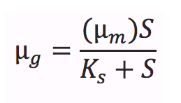
One important equation which has been incorporated into our model is the Monod equation. This equation is most commonly used to model microbial growth and has been shown to fit a large variety of empirical data[1]. In addition, it shares the key assumption described above. This equation relates the specific growth rate (µg, the increase in cell mass per unit time) as function of the maximum growth rate (µm), and the concentration of a limiting substrate (S). The equation is written as follows:
where KS is the limiting substrate concentration when the specific growth rate is at half maximum (KS = S when µg = µm/2). KS is also known as the saturation constant or half-velocity constant[1].
Contents |
Equations and Constants
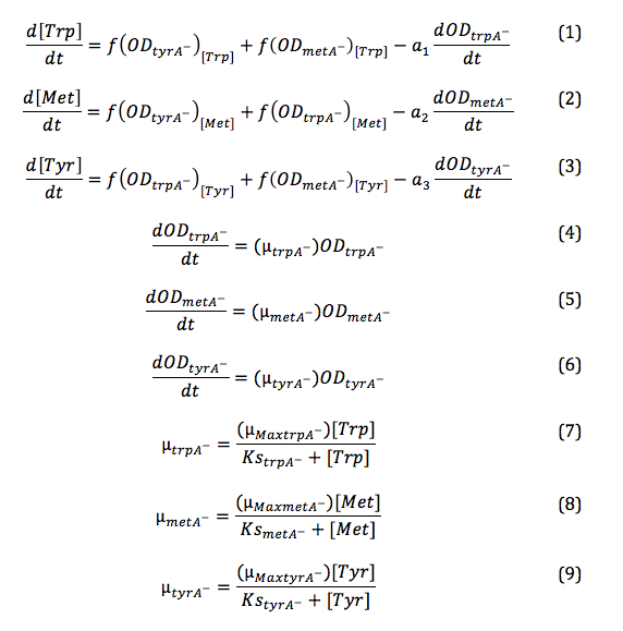
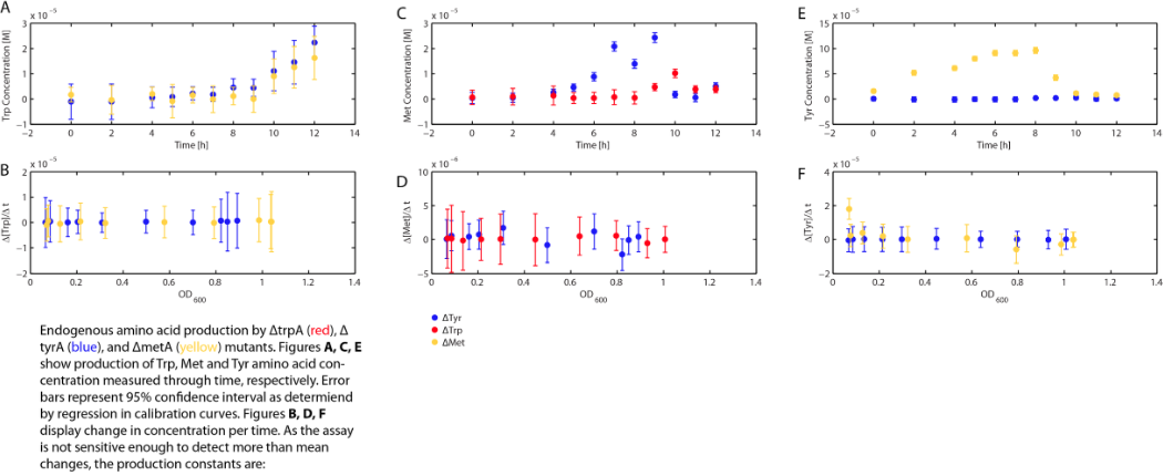
Applying the Monod kinetic model, we sought out to measure three variables: the concentration of tryptophan, methionine, and tyrosine in the media available for each specific auxotroph. We were also interested in how these concentrations vary with respect to time.
As there is very limited initial availability of each amino acid in the media, the ability of each auxotroph to grow in coculture demonstrated that the amino acids necessary for growth are being produced and exported from the cell, and that each auxotroph is feeding on the amino acids produced by the other cells in the consortium. For the sake of the model, we assumed that the environmentally released tryptophan, methionine, and tyrosine were only consumed by the respective auxotrophic strain.
Combining the above assumptions with Monod kinetics, we proposed the following fundamental equations for our consortium model. In this model, each auxotrophic strain is denoted with a superscript minus (i.e. ΔtrpA, ΔmetA, and ΔtyrA are denoted trpA-, metA-, and tryA-, respectively); [Trp], [Met], and [Tyr] represent the concentrations of tryptophan, methionine, and tyrosine; ODtrpA-, ODmetA-, and ODtyrA- represent the optical densities of the ΔtrpA, ΔmetA, and ΔtyrA strains; a1, a2, and a3 are the consumption constants with respect to changes in ODtrpA-, ODmetA-, and ODtyrA-, respectively; µtrpA-, µmetA-, µtyrA- are the specific growth rates of the ΔtrpA, ΔmetA, and ΔtyrA strains; µMaxtrpA-, µMaxmetA-, µMaxtyrA- are the maximum growth rates of the ΔtrpA, ΔmetA, and ΔtyrA strains; and KstrpA-, KsmetA-, KStyrA- are the half-velocity constants of the ΔtrpA, ΔmetA, and ΔtyrA strains. The terms and constants of this equation will be discussed in further detail later.
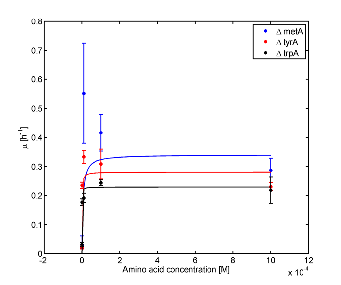
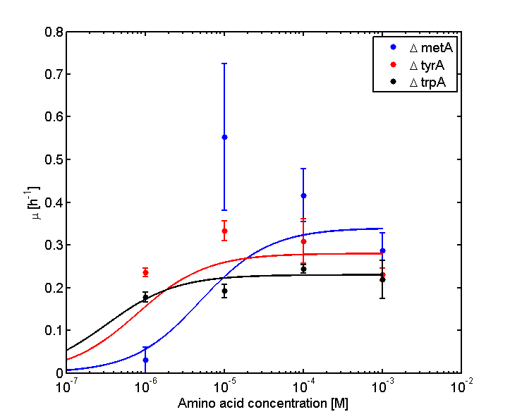
In the above equations, some of the key constants for the Monod Kinetics are obtained through analyzing the growth curves in a 96-well plate, with varying amino acid concentrations. Characteristic growth rates were observed and plotted:
Figure 1: Monoculture Growth Rates at various Limiting Amino Acid Concentrations
Figure 2: Log Scale of Monoculture Growth Rates at various Limiting Amino Acid Concentrations
note: we had lower amino acid concentrations designed as well, though we found out that when concentration is below 1E-7 M, cell OD over night does not show significant differences through out the incubation period. However, their OD do still varies, in the magnitude of 0.01, and is hard to differ from controls and is considered no growth and shown as the one of the error bars. For detailed protocol, please go to Link:….new protocol.
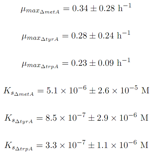
Based on Figure 1 and 2, key constants such as maximum growth rates, and half-velocity constants for each auxotrophs are obtained [1]:
Further more, as discussed in the beginning of this section, we assumed that the amino acid consumption is solely depended on the cell growth and not the cell self maintenance. In order to find out the remaining constants, consumption rate constants (a1, a2, and a3), we need to find out a way to measure the amino acid concentrations in the media with respect to the change of its OD for each auxotroph.
To do this, firstly, we need to find a way to measure media amino acids concentrations. With no good access to HPLC, we noticed in previous experiments that each of the knockout monocultures will reach to a certain final OD at a different known amino acid concentrations, and also according to a recently published paper: A Programmable Escherichia coli Consortium via Tunable Symbiosis, Kerner A et. al (2012) confirmed that there indeed is a relationship between the final auxotroph ODs with the environmental amino acid concentrations, though may not be very accurate[2].
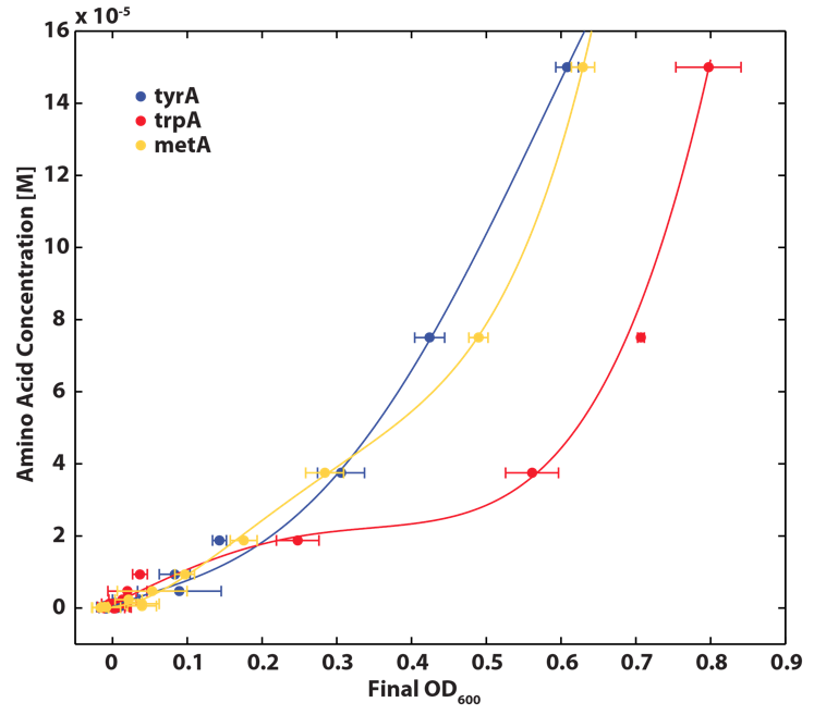
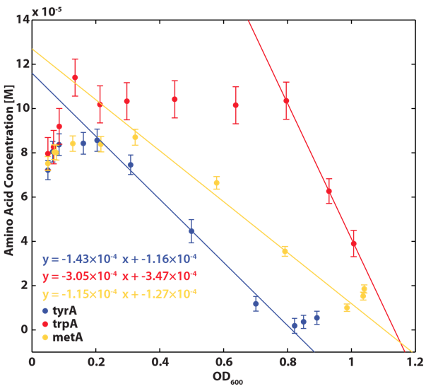
Thus we generated a calibration curve to relate the limiting amino acid concentrations to their final OD readings based on our own wet lab data for our specific ΔtrpA, ΔmetA, and ΔtyrA E. coli strains, which are shown in the figures below:
Figure 3: TrpA Auxotroph Final OD and Trp Concentration Calibration Curve
Figure 4: MetA Auxotrph Final OD and Met Concentration Calibration Curve
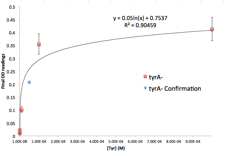
Figure 5: TyrA Auxotroph Final OD and Tyr Concentration Calibration Curve
Note: all the data are obtained through triplicates, and detailed protocol can be found in Link:……..new…protocol. Also, we tested the accuracy of one of the calibration curves. The blue dot in Figure 5 is another data value we obtained later at a known Tyrosine concentration (5E-5 M), and it is reasonably close to the predicted curve. This test point has proven that this calibration curve can serve us well at this stage of the research; however, we are aware that this curve has limitation, mainly due to the big error bars at the higher OD data points. For future accuracy improvement, more data points (more of the same concentrations as well as more of different concentrations) should be collected.
Secondly, it is necessary to find out how the amino acid in the environment is consumed with respect to cell growth.
We grew all three auxotrphs: ΔtrpA, ΔmetA, and ΔtyrA in 50 ml flasks with known initial Tryptophan, Methionine, and Tyrosine concentrations (5E-5 M) respectively, and harvested 5ml of cell free supernatants at various ODs. All these supernatants served as new 96-well plate media for each knock out cultures with newly added M9-Glucose shots (2% glucose in the well), which made sure the amino acids of interest remained as the limiting substrate for all knock outs. its detailed protocol can be found here.
After growing the inoculated 96-well plate in humidified temperature control (37 deg) plate reader for 15 hours, their growth curves had been captured and most of the monocultures had reached their stationary phase, and the plate was then transferred to 37 deg room to obtain the remaining final OD readings.
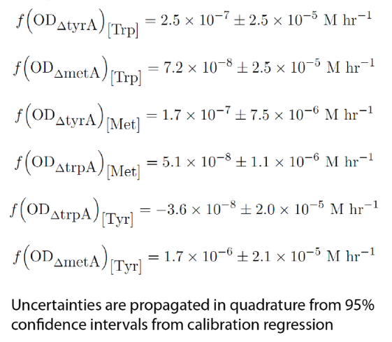
Based on the calibration curves (Figure 3, 4, 5), the amino acid concentrations in the wells were calculated from their final OD readings, and when corrected with a dilution factor of 5/4 (as we added in the 5X, it was 1/5 of the total well media volume, which is described here again), we arrived at the corresponding supernatant amino acid concentrations at various auxotroph monoculture OD readings. Again, with the assumption that the only change in the amino acid concentration in the media is due to cell growths, and as they are specific knock outs, they were not able to produce any amino acid into the environment, each auxotrophs' consumption constants with respect to cell growth rate (a1, 2, 3) can be calculated. Their values are:
Thirdly, after founding out the consumption constants for corresponding auxotrophs, we were interested in finding out how the other two auxotrophs will contribute to this specific amino acid changes in the environment. After all, these equations (f(ODtrpA-)s, f(ODmetA-)s, and f(ODtyrA-)s in equation (1), (2), and (3)) are the key to the accuracy of this model.
In the coculture environment, for the behaviour of auxotrophs with respect to changing the environment amino acid concentrations, the closest assumption we can make is that teach auxotrph will behave similarly to its behaviour in its monoculture condition. Thus, we used the same calibration curve for relating the final OD to the limiting substrate amino acid concentration in the media. The difference is that in stead of finding out the corresponding limiting amino acid concentration, e.g., ΔmetA media for [Met] measurements, this time, we are finding out the other two non-limiting amino acid concentrations of each knocked out E. coli auxotrophs, e.g. ΔmetA media for [Trp] and {Tyr] concentrations, at various OD readings [2]. With the consideration of sample taken time and some data manipulation, we were able to derive six functions that relate the change of all amino acid concentrations with respect to time (e.g. d[Trp]/dt), with the other two auxotrophs' optical densities (e.g. ODmetA- and ODtyrA-), which is shown below:
Note: all these equations have been previously mentioned in equation (1), (2), and (3), and can be directly substituted into them later to reduce the number of equations in the Matlab Code section.
One big limitation of the accuracy of these equations is that their accuracy is extremely dependent on the accuracy of the calibration curves (Figure 3, 4, and 5) as well as precision and accuracy of the OD readers, especially when OD readings are low. As you can see from Figure 3, 4, and 5, the slope is extremely high for all of them at low OD values, and thus are very sensitive to inaccurate low OD readings (OD<0.1).
However, some of the equations are derived from the available data assuming that at low OD values, it is still reasonable to use the calibration curve to calculate the supernatant (cell free media) amino acid concentration.
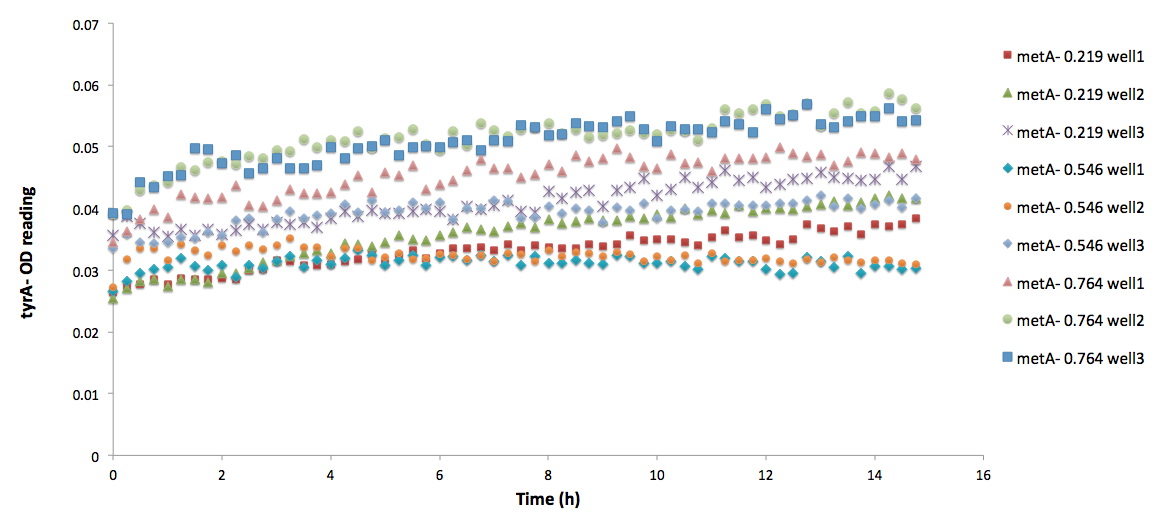
Especially for Equation (15), its raw experimental OD readings are shown below:
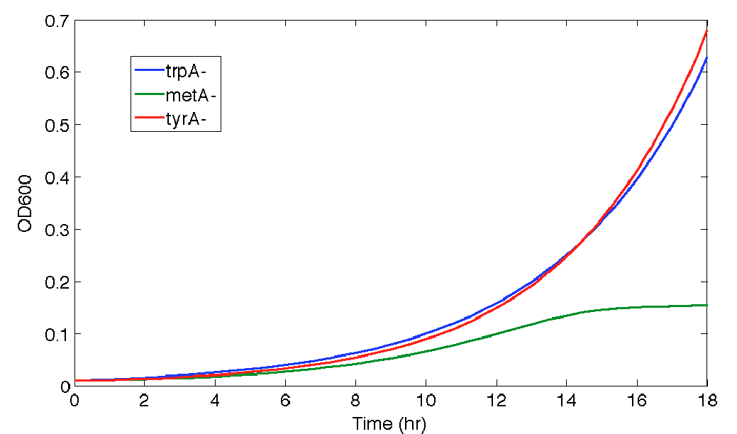
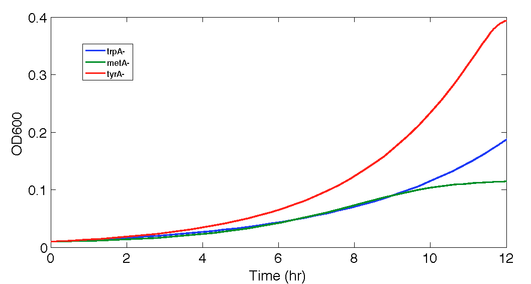
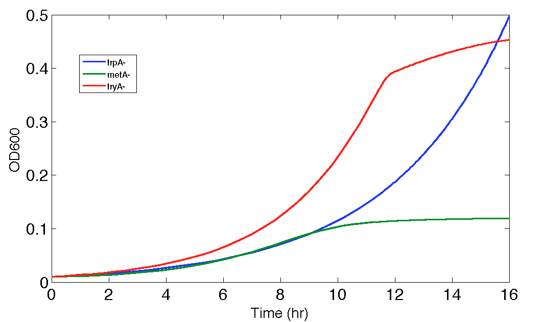
Figure 6: ΔtyrA auxotroph growth curve in various ΔmetA ODs cell free supernatants in 96-well plate reader environment
Note: As discussed before, all of this data can cause inaccurate supernatant concentration calculation due to its extremely low OD readings. All data sets are labelled correspondingly, where triplicates are noted by well 1, 2, and 3. As we can see, there are some distinct differences in the OD readings among the three different supernatant data sets; however, when corrected through focusing on the difference between the initial reading and the final reading with a base adjustment of 0.025 (which is the lower value used for all the calibration curves), they average roughly the same, with an average OD value of 0.03847, 0.04043, and 0.04218, respectively, for ODmet 0.219, 0.546, and 0.764. To make sure you understand this calculation fully, Here is a sample calculation: for example, suppose one set of the data has an initial OD reading of 0.02, and a final OD reading of 0.04, then we conclude that there is a difference/growth of (0.04-0.03)=0.01 OD of cells, and then it is corrected with the base OD reading, 0.025, for calibration curve applicability. Thus, it reaches a effective final OD of (0.025+0.01)=0.035. This process is replicated for all triplicates, and by averaging these three effective final ODs, the average OD value is used for concentration determination is arrived.
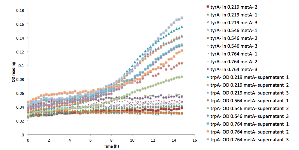
To demonstrate more clearly that this function (equation (15)) can be an outlier, here is a comparison with one other sets of growth curve that is run in the same plate by plotting them together.
Figure 7: ΔtyrA auxotroph growth curve in various ΔmetA ODs cell free supernatants in 96-well plate reader environment
Note: this set of data is not just any random data set. As you can see from the legend, both of the data sets are obtained as auxotrophs ( ΔtyrA and ΔtrpA) growing in the same supernatants that were obtained from ΔmetA growing media at various ODs. Also, to make it more obvious for readers to get a sense of raw data, it is shape labelled as triangles, circles, and squares for OD 0.219, 0.546 and 0.764 respectively.
It is easy to notice that all three of the trpA- sets of growth curve grew to a much higher OD (reaching about 0.17) at the end of 15 hours and was still growing, whereas all tyrA- sets grew significantly less, with an average initial and final OD differences of only about 0.01.
Matlab Code
Now with all the key functions and constants approximated, we are able to encode our model into Matlab, where the six key ODE functions can be solved and output the our prediction of population dynamics
The code is shown below, which contains a detailed step by step instruction for future iGEM teams or related scientific researches use, as well as the clarifications of our own code. It is also written is a way that it can be directly copied and pasted into Matlab blank m.files with all the comments in Matlab commenting format already, so that the coder can read the coded instructions and explanations in the coding command window without having to switching between, for example, the matlab and browser windows.
Of course, copying and pasting the code here is welcomed!
Code begins here:
% input the following commands, which are all in bold, into MATLAB command window, and not the m.file, before you call the ODE function.
%firstly, define a time array, set the upper limit to be the time (hr) you want this model to predict. For this model to be accurate, it is advised not to use extreme values.
%in our cases, the upper limit is set to 12 as some of the modelling equations are based on 11 hour culture supernatant data. Thus accuracy is expected within 12 hours.
% >> xspan = [0 12];
%in order to set up the initial conditions, where they corespond to the initial values of y(1), y(2), y(3)..., to y(6) in our case, and y(n) if you have n number of ODE equations
% >> ynot = [1E-7 1E-7 1E-7 0.01 0.01 0.01]';
% the first three values are the initial values for y(1), y(2), and y(3) respectively, which in out cases are the initial amino acid concentrations, and as we are adding the cells directly into the M9 media without supplementing any amino acids, it is believed to be at very low concentrations, and thus is set to 1E-7 mole/L.
% the remaining three values are the initial conditions for y(4), y(5), and y(6), which are the initial cell ODs in out case, and they are all set to 0.01, which is based on the lower values of the OD plate readings after correcting with blanks.
%Then RUN THE FUNCTION
% >>[X,Y] = ode45(@UBCiGEM2012_ConsortiaModel,xspan,ynot);
% this takes the function name in your m.file, the range of your interest, and the initial conditions which is just defined, respectively
%Note: have to make sure that the name is exactly the same as the function name in your m.file for it to be able to run correctly.
%the following code is for the actual mfile.
% 1) Declare the name of the function:
function dy = UBCiGEM2012_ConsortiaModel(t,y);
% 2) define all your ODE variables clearly for your own understanding as they can get quite confusing if you don't.
% in our case:
% y(1) = [Trp];
% dy(1) = d[Trp]/dt
% y(2) = [Met];
% dy(2) = d[Met]/dt;
% y(3) = [Tyr];
% dy(3) = d[Tyr]/dt;
% y(4) = [OD_trpA-];
% dy(4) = d[OD_trpA-]/dt;
% y(5) = [OD_tyrA-];
% dy(5) = d[OD_tyrA-]/dt;
% y(6) = [OD_metA-];
% dy(6) = d[OD_metA-]/dt;
% 3) define your constants first that will not depend on variables
% in our case, it was all measured through our own wet lab data and is explained in the previous section
%define maximum growth rate constants
u_maxtrpA = 0.2442; % units = hr-1
u_maxmetA = 0.5524; % units = hr-1
u_maxtyrA = 0.3332; % units = hr-1
%define half-velocity constants
Ks_trpA = 1E-7; % units = M
Ks_metA = 5E-6; % units = M
Ks_tyrA = 8.36E-8; % units = M
%define the consumption rate constants
a1 = 4.08E-4; %units= M/OD
a2 = 1.44E-4; %units= M/OD
a3 = 1.23E-5; %units= M/OD
% 4) write out ODE CODE, suggest to write out all equations on paper first, as they are a lot more clear than coding them directly, and will reduce the chance for you to make error why coding significantly.
dy = zeros(6,1);
dy(1) = ((1e-8)*(exp(1))^(16.586*y(4))) + ((-0.023*(y(5))^2)+0.021*y(5)-3.5e-3) - a1*(u_maxtrpA*(y(1))/(Ks_trpA+y(1)))*y(4);
dy(2) = ((9e-6)*(y(6))^2-(7e-6)*y(6)+1e-6) + (((2e-6)*(y(4))^2)-(2e-6)*y(4)+9e-7) - a2*(u_maxmetA*(y(2))/(Ks_metA+y(2)))*y(5);
dy(3) = ((3e-7)*(y(4))^2-(8e-7)*y(4)+4e-7) + (((1e-6)*(y(5))^2)-(2e-6)*y(5)+6e-7) - a3*(u_maxtyrA*(y(3))/(Ks_tyrA+y(3)))*y(6);
dy(4) = (u_maxtrpA*y(1))/(Ks_trpA+y(1))*(y(4));
dy(5) = (u_maxmetA*y(2))/(Ks_metA+y(2))*(y(5));
dy(6) = (u_maxtyrA*y(3))/(Ks_tyrA+y(3))*(y(6));
% note: For easy coding and checking purposes, all this equations are exactly the same as the one shown in equation (1), (2), and (3) for dy(1), dy(2), and dy(3) respectively, with also the same arrangements of each equation term within them.
% and Please also note: these equation has been derived with direct simple substitution of equations, where equation (4), (5), (6), (7), (8), (9), (10), (11), (12), (13), (14) and (15) have been substituted into the equation (1), (2) and (3).
%if you want, you can choose to plot diagrams and display the predicting dynamics within the m.file or manually plot the arrays of your interests in command window
%For example, for this project, we are interesting in predicting the ODs of each auxotrophs, thus, we manually plotted values in y(4), y(5), and y(6) (which again, are the OD values of each auxotrophs) agaisnt time, by typing the following in the command window after run the ODE45 functions:
%>>plot(X,Y(:,4:6))
End of the m.file
Note: I will indicate here that the direct translation of the previous discussed equations with simple substitutions at either the beginning or the end of this section
Simulation Results, Analysis and Future Work
When the Matlab Code was run, it generated a graphic result predicting the population dynamics without inducing, which is shown in the following diagram:
Figure 8. Population Dynamics Prediction within 12-hour Confidence Range
Figure 9. Population Dynamics Prediction for 16 hours
As we can see here, the prediction is no longer reasonable as the ΔtyrA OD shoot off into 1.8 after 16 hours of incubation.
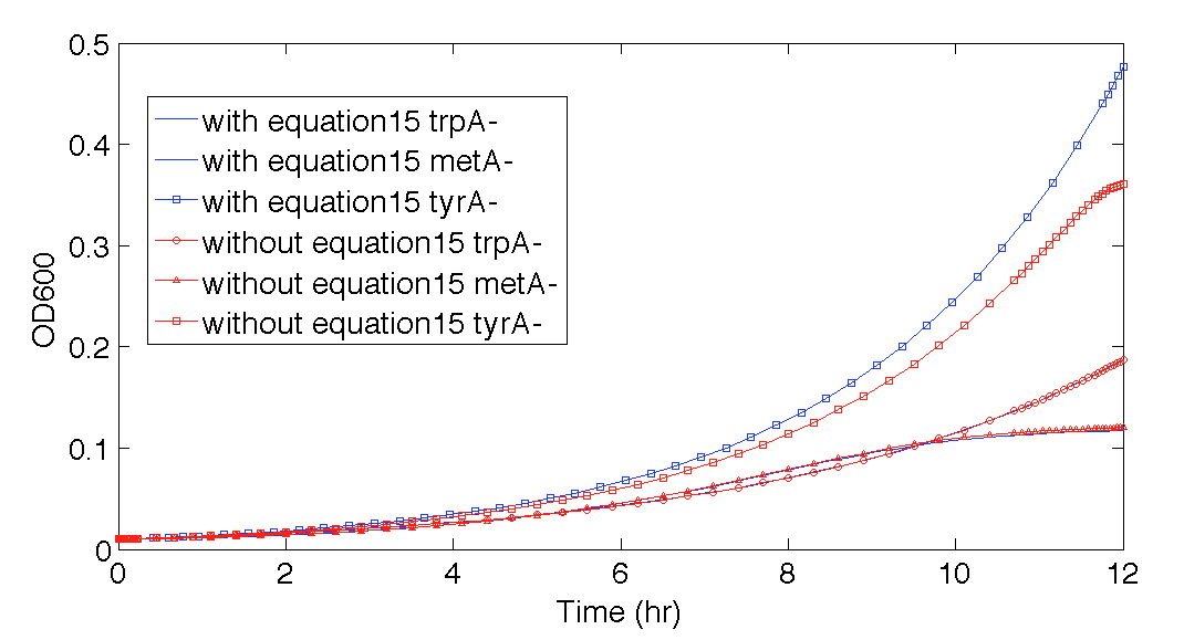
However, as we explained in the end of Equation and Constants section, equation (15) can be an outlier equation for this modelling, and the [Tyr] concentration is proven to be so low in the environment that we can barely observe any growth even with the precisions of an high-end plate reader.
Thus, we were very interested in finding out how the predictions would be differed if we took out equation (15) from the simulation code, as if we assumed the environment tyrosine concentration had no relationship with ΔmetA growth. The result of both 12 and 16 hour predictions are shown in Figure 10, and 11.
Figure 10. Population Dynamics 12-hour Prediction after eliminating one potential inaccurate function, equation (15)
Figure 11. Population Dynamics 16-hour Prediction after eliminating one potential inaccurate function, equation (15)
From these figures, it was not surprising to see that the prediction become reasonable again for 16 hours one too, as the sum of the ODs sum ups to about 1, which proved that the attempt of generating the functions to relate d[Tyr]/dt as a function of ODmetA- based on extremely small OD reading values, had more negative effect on the accuracy of the modelling than assuming that the growth related tyrosine production or consumption of the environment was so insignificant and could thus be assumed to be zero (d[Tyr]/dt= f(ODmetA-)tyr=0).
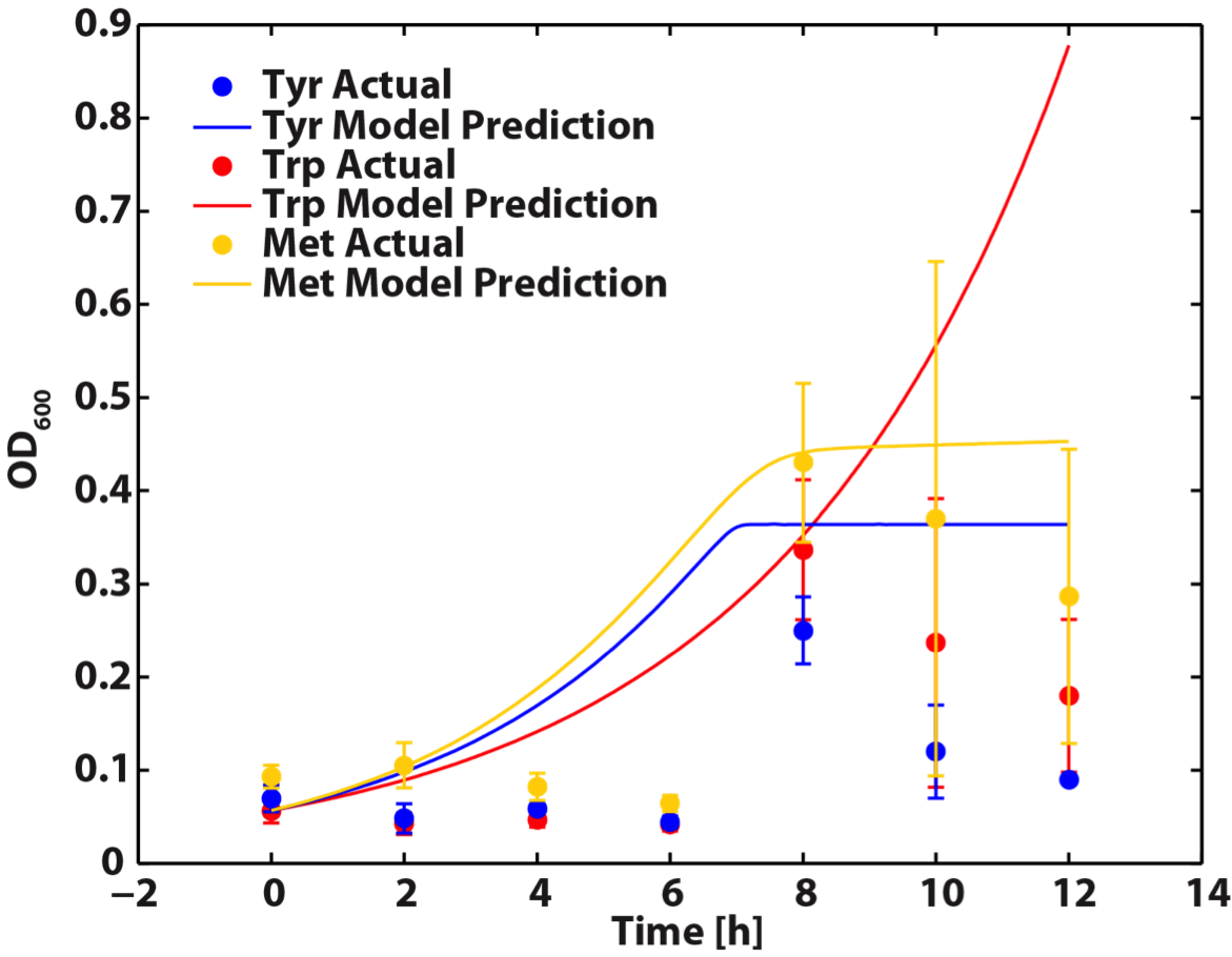
Also, please note that the 12 hour prediction with this equation elimination (Figure 11) is almost identical to the prediction when equation (15) is still in the code, where the effect of equation (15) can be better visualized in Figure 12. This also confirmed that when the time was with 12 hours, this modelling could work reasonably well, even if some of the equations used was not accurate, it was empirically accurate within our confidence range at least.
Figure 12. Population Dynamics 12-hour predictions with and without eliminating one potential inaccurate function, equation (15)
Thus, for future work, now that we have demonstrated that our model can work, and we can make it even better if we have more qualitative/accurate data, or more quantitive data (more data to generate more accurate calibration or function curves) in general. It can be done through running the generation of amino acid experiment with more of OD of interest, or, instead of using the final OD calibration curves, we can try with another more accurate and direct measurement of the supernatant amnio acid concentrations, such as HPLC.
Also, we can set up experiments to test the accuracy of the population dynamics through taking samples at various time of the coculture flasks and scan the sample using fluorscence reader to get the real population dynamics in the actual consortia, and compare it with this modelling prediction (now our wet lab consortium population dynamic data are solely based on 96-well plate environment).
Lastly, as mentioned at the description, this code can be generalized to predict the population dynamics when there is a tuning effect, as long as we can generate six new functions describing the amino acid dynamics in each monoculture. Therefore, we can use this model to decide the amount of tuning (by adding in different amount of inducer) needed to obtain the desired relative population of each auxotrophs.
References
[1] Shuler, ML; Kargi, F; Bioprocess Engineering Basic Concepts, 2002 2nd edition. Prentice Hall PTR.
[2] Kerner A; Park J; Williams A; Lin XN; A Programmable Escherichia coli Consortium via Tunable Symbiosis, 2012. PLoS ONE 7(3): e34032. doi:10.1371/journal.pone.0034032
 "
"
