Detail Calculation Method and Results

Contents 1 Calculation and Derivation of the Protein Expression Amount Model in Three States 1.1 Overview 1.2 Input of Our Calculation 1.2.1 RBS sequence 1.2.2 16S rRNA sequence 1.3 Formula Derivation 1.3.1 Basic Idea 1.3.2 Basic Assumption 1.3.3 Formula Derivation 1.4 The Calculation 1.4.1 Control State (c) 1.4.2 Experimental state 1 (E1) 1.4.3 Experimental state 2 (E2) 1.4.4 The Calculation of ΔGtot 1.5 Calculation Results of ΔG 1.6 Prediction of Protein Expression Amount 1.7 Model Extension 2 Analytical hierarchy process (AHP) 2.1 What is AHP? 2.2 Is there any application in real life? 2.3 The AHP procedure 2.4 Calculation result through AHP method 2.4.1 IGEM Project evaluation model 2.4.2 Determination of the Optimum propaganda method 2.4.3 Universal Risk evaluation model of Environmental problem 2.5 Reference 3 Principal component analysis (PCA) 3.1 What is the problem? 3.2 What is principal component analysis? 3.3 How to use PAC? 3.3.1 Determine the Objectives? 3.3.2 How to start? 3.3.3 Determining the number of components 3.3.4 How to get the principal components 3.3.5 Mathematical background on principal component analysis 3.3.6 Algorithms 3.4 Reference

Calculation and Derivation of the Protein Expression Amount Model in Three States

Overview

Three problems came up while we start calculating: what sequences to input, which method to use and how cogent the result will be. As for sequence, we input the both the SD and the protein coding sequence.

Our goal is to calculate the total ΔG of each reaction and then predict the amount of protein expressed. There are several softwares dealing with DNA or RNA base-pairing progress, such as NUPACK, RBS-Calculator, and Vienna RNA etc. After comparison, we decide to use RBS-Calculator.

Due to the complication of translation progress and our lack of insight in this issue, the results of our modeling can’t be very precise. But at least it should have the precision of order of magnitude.

Input of Our Calculation

RBS sequence

• RFP, normal RBS

ATTTCACACATACTAGAGAAAGAGGAGAAATACTAGATGGCTTCCTCCGAAGACGTTATCAAAGAGTT

CATGCGTT

• RFP, orthogonal RBS

ATTTCACACATGTTCCGTACTAGATGGCTTCCTCCGAAGACGTTATCAAAGAGTTCATGCGTT

• GFP, normal RBS

TACTAGAGAAAGAGGAGAAATACTAGATGCGTAAAGGAGAAGAACTTTTCACTGGAGTTGTCCCAAT

TCTTGTT

16S rRNA sequence

• normal 16S: ACCTCCTTA
• orthogonal 16S: ACGGAACTA

Formula Derivation

Basic Idea

For model design, please refer to Design part. Data of the curve Er-time is obtained from E_c=K∙E_r experiments. The function of our model is to work out the proportion factor 'K'.

Basic Assumption

1. The expression of RFP and GFP are independent.
2. The expression of the two proteins are determined by the percentage of normal and orthogonal ribosomes rather than the number of the two ribosomes.
3. The growth curve of bacteria do not change significantly after the transferred into orthogonal protein expression system.

Formula Derivation

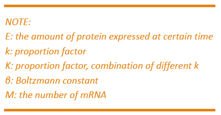
We start from Formula 1 and 2. In Formula 1, m stands for the number of mRNA transcript, R_tot is the total number of ribosomes, β is the apparent Boltzmann constant, ∆G_tot is the total change of Gibbs free energy, k is proportion factor.

Because the GFP and RFP coding sequence are on the same mRNA transcript, the values of m of GFP and RFP are always same. In different state and time, the total number of ribosomes varies. We assume that at the same time R_tot of different state remain same. Calculation of DG_tot is the main job of this model. The proportion factor 'k' represents all unknown factors. Here we assume that as for the same protein in deferent state 'k' varies little.

The Calculation

Control State (c)

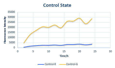
The two formulas above serve as denominators in following deduction. We get series of disjointed data of Function 3 and 4 through experiments. The amount of GFP and RFP can't be measured directly so we measured the fluorescence intensity of each protein. And because all the formula in this model are based on a singular cell, we must consider the influence caused by the number and growing condition of bacteria.

Experimental state 1 (E1)

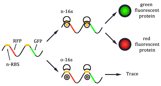
The expression of GFP is composed of two part, the expression of n-RBS::n-16S and of n-RBS::o-16S.

There is no difference for the expression of GFP in Experimental state ONE from the control state, except for the distribution of ribosomes. For this reason, we presume that kc1,G and kr,G are nearly equal and thus Kc1,G equal to 1. The same thought is also shown in following derivation.

We noticed that the proportion factors in equation 6 and 8 are equal, which is not a coincident. This is because ΔG_3,G-ΔG_1,G≈ΔG_3,R-ΔG_1,R. The difference of ΔG_3,G and ΔG_1,G.

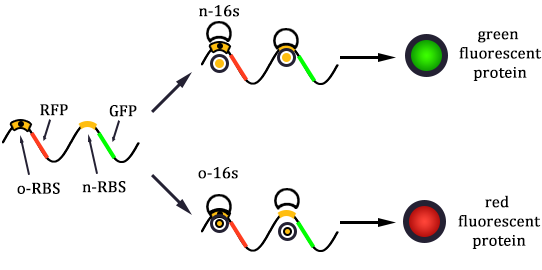
Experimental state 2 (E2)

Note : Strictly speaking, the factor K should better be obtained from experimental data rather than assumed to be 1 for such simplification could lead to much deviation from real value.

The Calculation of ΔG_tot

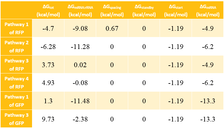
In most cases, the difference of delta G among the four pathways are mainly reflected by the ΔG_mRNA-rRNA. There are two ways to calculate the ΔG_mRNA-rRNA:

1. With the help of RBS calculator;
2. Use the method in literature Computational design of orthogonal ribosomes.

There are some differences between the input and output of the two method.

1st method:

• input:
  • standby + RBS + Spacing + Start Codon + Protein-Coding,
  • 16S 3' last nine bases;
• output: ΔG_mRNA:rRNA, ΔG_start, ΔG_spacing, ΔG_standby, ΔG_mRNA;
• Software: RBS-Calculator;
• Strength: taking more factors into our consideration and are more accessible to real condition;
• Weakness: not sure of the input sequence.

2nd method:

• input:
  • ASD sequence,
  • SD sequence (each are 6 bases long);
• Output: ΔG under different conditions;
• Software: RNA-Cofold in Vienna RNA web servers;
• Strength: only need to input the SD and ASD sequence which is very easy;
• Weakness: not as accurate as the first method.

Similarity of the two method：The core program of RBS-Calculator is based on Vienna RNA.

There are also two points that should be focused on during our modeling:

1. the specification of input;
2. the analysis of errors if there are any in the output.

As for analysis of errors, the most frequent errors are the Long-Range Paring which occurred when the head and the tile of the mRNA sequence complement with each other within the sequence itself. In such case, the ΔG_mRNA result is not accurate. We usually use RNA-Fold to calculate the accurate ΔG_mRNA to avoid such error.

Calculation Results of ΔG

Prediction of Protein Expression Amount

We should, first of all, measure the relative protein expression amount (fluorescence intensity) and to obtain the parameters in the model through regression. After the obtaining the model parameters, we can predict the amount of protein expressed and to compare them with that of wet lab results.

With the calculation result from the previous relative expression formula, together with the wet lab result of fluoresce intensity of RFP which is mentioned in the notebook, we can have the exact value of percentage of normal ribosome x.

After the calculation, we can obtain that x=0.9737, y=0.0263.

When determine the relative expression level, the GFP intensity should be the same for experiment state one and state two. However, there are some divergences between the GFP intensity of a single cell between the two states. We rationally assume the divergence in the total intensity is result from the number of bacteria (in other words, the OD value leads to the different GFP intensity). So the intensity of RFP for a single cell should also be adjusted.

We can put the value of x and y into the formula of the relative protein expression ratio. What is more, we also measured the Florence intensity curve of the control state. With the obtained value of the ratio we have predicted the curve of the experimental state one and the experimental state two. The result figure of our prediction process is shown in the following four figures.

Model Extension

In the previous protein expression model, we just suppose the existence of the orthogonal expression system do not have any significant impact on our system. However, to make our system more accurate, we also need to take the factor of estimation.

Analytical hierarchy process (AHP)

What is AHP?

The analytic hierarchy process (AHP) is a structured technique for organizing and analyz-ing complex decisions. Based on mathematics and psychology, it was developed by Thomas L. Saaty in the 1970s and has been extensively studied and refined since then.

It has particular application in group decision making, and is used around the world in a wide variety of decision situations, in fields such as government, business, industry, healthcare, and education.

Rather than prescribing a "correct" decision, the AHP helps decision makers find one that best suits their goal and their understanding of the problem. It provides a comprehensive and ra-tional framework for structuring a decision problem, for representing and quantifying its ele-ments, for relating those elements to overall goals, and for evaluating alternative solutions.

Is there any application in real life?

While it can be used by individuals working on straightforward decisions, the Analytic Hierarchy Process (AHP) is most useful where teams of people are working on complex problems, especially those with high stakes, involving human perceptions and judgments, whose reso-lutions have long-term repercussions. It has unique advantages when important elements of the decision are difficult to quantify or compare, or where communication among team members is impeded by their different specializations, terminologies, or perspectives.

Decision situations to which the AHP can be applied include:

• Choice - The selection of one alternative from a given set of alternatives, usually where there are multiple decision criteria involved.
• Ranking - Putting a set of alternatives in order from most to least desirable
• Prioritization - Determining the relative merit of members of a set of alternatives, as opposed to selecting a single one or merely ranking them
• Resource allocation - Apportioning resources among a set of alternatives
• Benchmarking - Comparing the processes in one's own organization with those of other best-of-breed organizations
• Quality management - Dealing with the multidimensional aspects of quality and quality improvement
• Conflict resolution - Settling disputes between parties with apparently incompatible goals or positions

The AHP procedure

Users of the AHP first decompose their decision problem into a hierarchy of more easily comprehended sub-problems, each of which can be analyzed independently. The elements of the hierarchy can relate to any aspect of the decision problem—tangible or intangible, carefully measured or roughly estimated, well- or poorly-understood—anything at all that applies to the decision at hand.

Once the hierarchy is built, the decision makers systematically evaluate its various elements by comparing them to one another two at a time, with respect to their impact on an element above them in the hierarchy. In making the comparisons, the decision makers can use concrete data about the elements, but they typically use their judgments about the elements' relative meaning and importance. It is the essence of the AHP that human judgments, and not just the underlying information, can be used in performing the evaluations.

The AHP converts these evaluations to numerical values that can be processed and compared over the entire range of the problem. A numerical weight or priority is derived for each element of the hierarchy, allowing diverse and often incommensurable elements to be compared to one another in a rational and consistent way. This capability distinguishes the AHP from other decision making techniques.

In the final step of the process, numerical priorities are calculated for each of the decision alternatives. These numbers represent the alternatives' relative ability to achieve the decision goal, so they allow a straightforward consideration of the various courses of action.

Several firms supply computer software to assist in using the process.

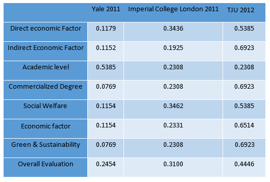
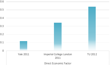
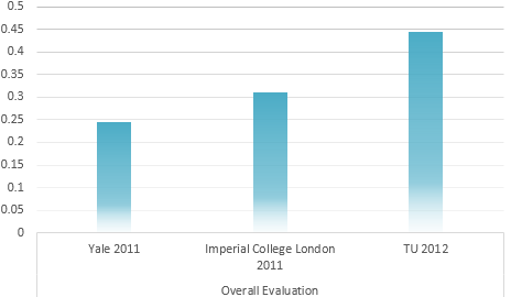
Calculation result through AHP method

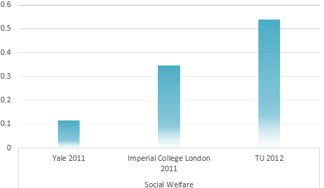
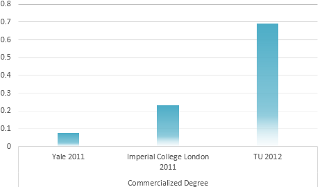
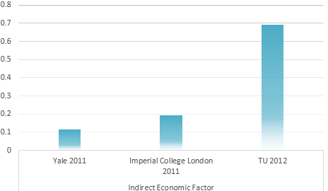
IGEM Project evaluation model

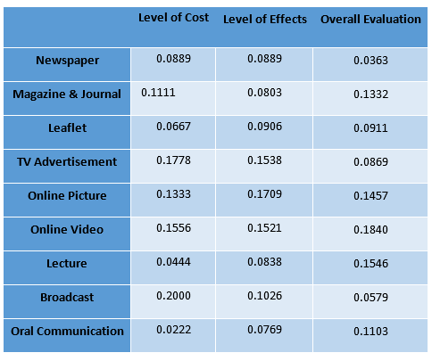
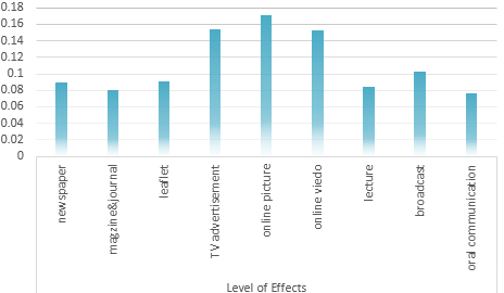
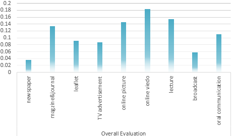
Determination of the Optimum propaganda method

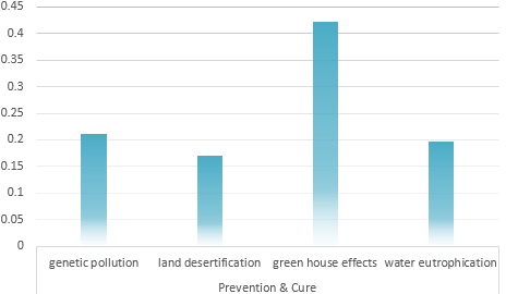
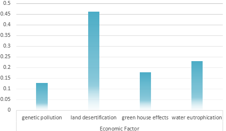
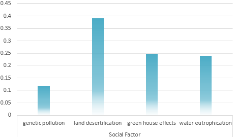
Universal Risk evaluation model of Environmental problem

Reference

1. Saaty, Thomas L.; Peniwati, Kirti (2008). Group Decision Making: Drawing out and Rec-onciling Differences. Pittsburgh, Pennsylvania: RWS Publica-tions. ISBN 978-1-888603-08-8.
2. Saaty, Thomas L. (2008-06). Relative Measurement and its Generalization in Decision Making: Why Pairwise Comparisons are Central in Mathematics for the Measurement of Intangible Factors - The Analytic Hierarchy/Network Process. RACSAM (Review of the Royal spanish Academy of Sciences, Series A, Mathematics) 102 (2): 251–318. Retrieved 2008-12-22.
3. Bhushan, Navneet; Kanwal Rai (January 2004). Strategic Decision Making: Applying the Analytic Hierarchy Process. London: Springer-Verlag. ISBN 1-85233-756-7.
4. Forman, Ernest H.; Saul I. Gass (2001-07). The analytical hierarchy processan exposition. Operations Research 49 (4): 469–487. doi:10.1287/opre.49.4.469.11231.

Principal component analysis (PCA)

What is the problem?

In assessing the main reasons of how the genetic pollution impact the world, we can analyze it from different perspectives, and the evaluation indexes are too numerous and complicated.

To make our assessing task easier, we need to classify all these evaluation indexes into various independent types according to the inherent characteristics of the indexes themselves. This is also called dimensionality reduction which can simplify our problem into various types. Through classification, we can also evaluate our projects through different independent perspectives. What is more, this type of classification can also provide some basic knowledge to classes.

After the classification we can not only analyze the problems from the main per-spective which avoid the trouble of assessing the same problem from too many indexes, we can also know the performance of one problem in different single prospects.

As for how to accomplish this task, we need to use the principal component analysis (PCA) method.

What is principal component analysis?

Principal component analysis (PCA) is a mathematical procedure that uses an orthogonal transformation to convert a set of observations of possibly correlated variables into a set of values of linearly uncorrelated variables called principal components. The number of principal components is less than or equal to the number of original variables. This transformation is defined in such a way that the first principal component has the largest possible variance (that is, accounts for as much of the variability in the data as possible), and each succeeding component in turn has the highest variance possible under the constraint that it be orthogonal to (i.e., uncorrelated with) the preceding components. Principal components are guaranteed to be independent only if the data set is jointly normally distributed. PCA is sensitive to the rela-tive scaling of the original variables. Depending on the field of application, it is also named the discrete Karhunen–Loève transform (KLT), the Hotelling transform or proper orthogonal de-composition (POD).

PCA was invented in 1901 by Karl Pearson. Now it is mostly used as a tool in exploratory data analysis and for making predictive models. PCA can be done by eigenvalue decompo-sition of a data covariance (or correlation) matrix or singular value decomposition of a data matrix, usually after mean centering (and normalizing or using Z-scores) the data matrix for each attribute. The results of a PCA are usually discussed in terms of component scores, sometimes called factor scores (the transformed variable values corresponding to a particular data point), and loadings (the weight by which each standardized original variable should be multiplied to get the component score).

PCA is the simplest of the true eigenvector-based multivariate analyses. Often, its operation can be thought of as revealing the internal structure of the data in a way that best explains the variance in the data. If a multivariate dataset is visualized as a set of coordinates in a high-dimensional data space (1 axis per variable), PCA can supply the user with a low-er-dimensional picture, a "shadow" of this object when viewed from its (in some sense) most informative viewpoint. This is done by using only the first few principal components so that the dimensionality of the transformed data is reduced.

PCA is closely related to factor analysis. Factor analysis typically incorporates more domain specific assumptions about the underlying structure and solves eigenvectors of a slightly different matrix.

How to use PAC?

Principal component analysis (PCA) involves a mathematical procedure that transforms a number of (possibly) correlated variables into a (smaller) number of uncorrelated variables called principal components. The first principal component accounts for as much of the var-iability in the data as possible, and each succeeding component accounts for as much of the remaining variability as possible.

Determine the Objectives?

Generally, there are two objectives of the PAC listed in the following:

• To discover or to reduce the dimensionality of the data set;
• To identify new meaningful underlying variables.

How to start?

We assume that the multi-dimensional data have been collected in a Table Of Real data matrix, in which the rows are associated with the cases and the columns with the variables. Traditionally, principal component analysis is performed on the symmetric Covariance matrix or on the symmetric Correlation matrix. These matrices can be calculated from the data matrix. The covariance matrix contains scaled sums of squares and cross products. A correlation matrix is like a covariance matrix but first the variables, i.e. the columns, have been standardized. We will have to standardize the data first if the variances of variables differ much, or if the units of measurement of the variables differ. You can standardize the data in the Table Of Real by choosing Standardize columns. To perform the analysis, we select the Tabel Of Real data matrix in the list of objects and choose To PCA. This results in a new PCA object in the list of objects. We can now make a scree plot of the eigenvalues, Draw eigenvalues to get an indication of the importance of each eigenvalue. The exact contribution of each eigenvalue (or a range of ei-genvalues) to the "explained variance" can also be queried.

Determining the number of components

There are two methods to help you to choose the number of components. Both methods are based on relations between the eigenvalues.

• Plot the eigenvalues, Draw eigenvalues. If the points on the graph tend to level out (show an "elbow"), these eigenvalues are usually close enough to zero that they can be ignored;
• Limit the number of components to that number that accounts for a certain fraction of the total variance. For example, if you are satisfied with 95 of the total variance explained then use the number you get by the query Get number of components (VAF) no less than 0.95.

How to get the principal components

Principal components are obtained by projecting the multivariate data vectors on the space spanned by the eigenvectors. This can be done in two ways:

1. Directly from the Table Of Real without first forming a PCA object. You can then draw the Configuration or display its numbers.
2. Select a PCA and a Table Of Real object together and choose. In this way you project the Table Of Real onto the PCA's eigen space.

Mathematical background on principal component analysis

The mathematical technique used in PCA is called eigen analysis: we solve for the eigenvalues and eigenvectors of a square symmetric matrix with sums of squares and cross products. The eigenvector associated with the largest eigenvalue has the same direction as the first principal component. The eigenvector associated with the second largest eigenvalue determines the direction of the second principal component. The sum of the eigenvalues equals the trace of the square matrix and the maximum number of eigenvectors equals the number of rows (or columns) of this matrix.

Algorithms

If our starting point happens to be a symmetric matrix like the covariance matrix, we solve for the eigenvalue and eigenvectors by first performing a Householder reduction to tridiagonal form, followed by the QL algorithm with implicit shifts.

If, conversely, our starting point is the data matrix A, we do not have to form explicitly the matrix with sums of squares and cross products, A′A. Instead, we proceed by a numerically more stable method, and form the singular value decomposition of A, U Σ V′. The matrix V then contains the eigenvectors, and the squared diagonal elements of Σ contain the eigenvalues.

Reference

1. Pearson, K. (1901). "On Lines and Planes of Closest Fit to Systems of Points in Space" (PDF). Philosophical Magazine 2 (6): 559–572.
2. Abdi. H., & Williams, L.J. (2010). "Principal component analysis.". Wiley Interdisciplinary Reviews: Computational Statistics, 2: 433–459.
3. Shaw P.J.A. (2003) Multivariate statistics for the Environmental Sciences, Hod-der-Arnold. ISBN 0-340-80763-6.[page needed]
4. http://www.fon.hum.uva.nl/praat/manual/Principal_component_analysis.html