Introduction

    Home

    Team

Project Overview

    Hacking Systems

    Human Pratices

    Lab Diary

    Safety

Plasmid Plug&Play

    Introduction

    Background

    Experiments

    Modeling

    Results

    Parts

Associative Memory
     Network

    Introduction

    Background

    Experiments

    Modeling

    Results

Extras

    SynbioBrasil

    USP and Unesp

    Attributions

    Sponsors

    Acknowledgements

    Photos

Contents 1 Objective 2 Model 2.1 Estimation of the variables 2.1.1 Plasmid concentration 2.1.2 Estimating Recombinase Concentration. 2.1.3 ORF concentration 3 Results 4 Discussion 5 Appendix 5.1 Equations 6 References

Objective

In order to evaluate the feasibility of our project, we developed a mathematical model based on kinetic equations to simulate our experimental design. We consider important to approach this problem mathematically in order to evaluate some biological issues. Firstly, we evaluated the effect of linear DNA degradation when a ORF (open reading frame from a target gene) is inserted in bacteria after eletroporation. Secondly, we estimated the amount of DNA that should be amplified by PCR to optimize the recombination between the lox sites. We compared the results obtained from two recombination proteins: CRE and FLP. Finally, we discussed methodologies to improve our design using the standard biological parts.

Model

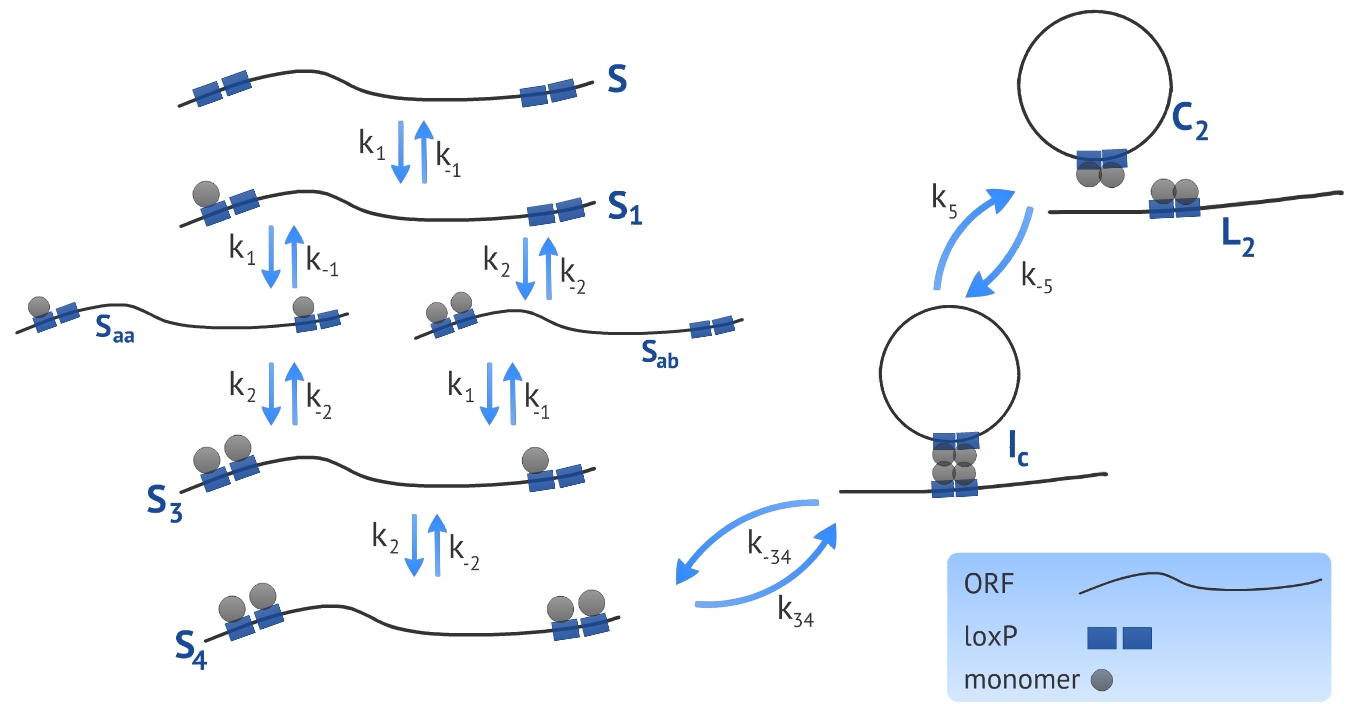
We developed a model based on the already proposed by Ringrose et al [1]. The authors introduced a model to describe a excision recombination reaction illustrated in Fig. 1. We used the parameters characterized by the authors in order to simulate our experimental design that consists in the circularization and insertion of the ORF in the Plug&Play plasmid. We also introduced a linear DNA degradation rate in the model in order to be more accurate in simulating in vivo process.

The first step when making a model based on kinetic equations is to determine the states or configurations of the system. In our context, we refer to S the linear ORF without any monomer bound and to S_a the linear ORF with one monomer bound, see Fig. 1. All four monomer sites (two sites per loxP) have the same affinity for the monomers, resulting in a symmetry in the system in terms of energy of association. Because of this, there is no need of distinguishing the site that the first monomer binds, referred as S_a. To represent the next state - the DNA bound by two monomers - we need to distinguish between two possibilities: there can be one monomer in each loxP, represented by S_aa, or two monomers in the same loxP, represented by S_ab. It is essential to distinguish these two states because the affinity of the monomers for the target site is different if there is already one monomer bound to the neighbor site. The following states representing the ligation of third and fourth monomer - referred as S₃ and S₄, respectively - have the same affinity and there is no need of distinguishing between them.

The rate of change at each state over time was approached by using kinetic equations. To illustrate this process, we described the kinetic equation which refers to the change of the state S over time:

\begin{align} &\frac{d}{dt}[S] = k_{-1}[S_{a}] - k_{1}[M][S] \end{align}

where M represents the concentration of recombinase monomers, k₁ and k₋₁ represents the association and dissociation rate constant, respectively. As described in the above equation, there is only two possibilities of changing the concentration of the state S: it can increase (positive sign) if a molecule in the state S_a loses the monomer or it can decrease (negative sign) if a monomer binds the DNA.

Using gel mobility shift assays it is possible to estimate the affinity of the monomer for their target site, represented by the parameters k₋₁ and k₁, as described by Ringrose et al [1]. They also estimated, using the same proceeding, the parameters k₋₂ and k₂ referring to the association and dissociation rate constant of the monomer for a target site when the neighbor site is already occupied by another monomer. Other parameters (k₃₄, k₋₃₄, k₅ and k₋₅) were determined by the authors comparing the simulated and in vitro recombination data, see Table 1.

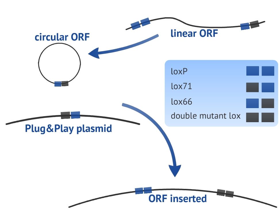
Our experimental design consists in a circularization of the ORF and its insertion in the Plug&Play plasmid. The circularization and insertion process are illustrated in figure 1 and 2, respectively. The equations of our model are presented in the appendix.

Estimation of the variables

In order to simulate our design, we defined the initial condition of our system, which consists in estimating the following variables:

• [P]₀ - initial concentration of the Plug&Play plasmids inside the bacteria.
• [M]₀ - initial concentration of recombinase monomers.
• [S]₀ - initial concentration of ORF inside the bacteria

To estimate the concentration of the variables, we need the volume of E. coli. According to [2] $V_{ec} = 0.7 \hspace{0.2cm}(\mu m)^3 = 0.7$ $10^{-15} L$. Using this estimation, it is possible to calculate the concentration of one molecule inside the bacteria in molar concentration
1M = 1mol / 1L = 6*10²³molecules / L

\begin{align} [1 molec] = \frac{1}{0.7*10^{-15} L} = \frac{1}{6*10^{23} 0.7*10^{-15}}M \simeq 1 nM \end{align}

Plasmid concentration

According to [3] it is expected approximately 100-300 plasmid inside the bacteria (high copy) and approximately 10 plasmids (low copy). So, using the equation we have:

• $[P]_0 \simeq 10 nM$ - high copy plasmid.
• $[P]_0 \simeq 100 nM$ - low copy plasmid.

Estimating Recombinase Concentration.

To estimate the concentration of recombinase we used a simple model:

\begin{align} &\frac{d}{dt}[mRNA] = \frac{k_{transc}}{V n_{bp}} - k_{dRNA}[mRNA] \end{align} \begin{align} &\frac{d}{dt}[Prot] = \frac{k_{transl}[mRNA]}{n_{aa}} - k_{dProt}[Prot] \end{align}

where the constant k_transl represents the translation rate, V refers to the volume of bacterium, n_bp refers to the number of base pairs of the protein, k_dRNA represents the mRNA degradation rate, k_transl represents the translation rate, n_aa the number of amino acids of the protein and k_dProt the degradation rate of the protein.

The values of these constants, obtained in [2] and [3], are presented below:

• $k_{degRNA} = 1/350$ (1/sec).
• $k_{transc} = 40$ (bp/sec) - for T7 promoter.
• $k_{transl} = 15$ (aa/sec).
• $k_{degProt} = 0.0167/60$ (Prot/sec) Average protein degradation.
• $n_{bp} = 1032 $ - for CRE.
• $n_{aa} = n_{bp}/3 = 344 $ - for CRE.
• $n_{bp} = 1119 $ - for FLP.
• $n_{aa} = n_{bp}/3 = 373 $ - for FLP.

Once we want the concentration of the protein in the equilibrium state, both equations are equal to zero:

\begin{align} \frac{d}{dt}[mRNA] = 0 \end{align} \begin{align} \frac{d}{dt}[Prot] = 0 \end{align}

and as a consequence:

\begin{align}\frac{k_{transc}}{V.n_{bp}} - k_{dRNA} .[mRNA] = 0 \end{align} \begin{align}\frac{k_{transl}[mRNA]}{n_{aa}} - k_{dProt} [Prot] = 0 \end{align}

So, an estimative of protein concentration per Plug&Play plasmid, for both CRE and FLP recombinases, is given by:

\begin{align} [Prot] = \frac{k_{transl} k_{transc}}{k_{dProt} k_{dRNA} n_{bp}^2/3 } \simeq 2000 nM \end{align}

This result is an estimation of the amount of protein (CRE or FLP) produced by each Plug&Play plasmid and consequently, the total concentration should be higher than 2000 $nM$ and dependent of the kind of Plug&Ply plasmid (high or low copy). Therefore, there is no significant change in the results presented here for concentrations higher than 2000 $nM$. This might occur because there are plenty of recombinase monomers to perform the recombination for concentrations higher than 2000 $nM$. Because of this, the following results are presented using 2000 $nM$ of monomer concentration.

ORF concentration

Estimate the ORF concentration inside the bacteria ([S]₀) is not simple because we do not know the amount of DNA that will get inside the bacteria during eletroporation. So we introduced a variable - lets call c - so that [S]₀ = c[So] represents the concentration, in average, of ORF copies inside the bacteria. The variable [So] represents the concentration of the DNA (ORF) in the solution before eletroporation and c is a constant such that c ≤ 1. In the most optimist scenario we have c = 1 which means that during eletroporation the concentration of DNA (ORF) inside the bacteria becomes the same as in the solution.

We can correlate the variable [So] with the amount of mass of DNA using the following relation: \begin{align} [So] = \frac{n_{mols}}{V} \end{align} where \begin{align} n_{mols} = \frac{m_{dna}}{n_{bp} m_{bp} n_{av}} \end{align} where m_dna is the mass of DNA, n_bp is the number of base pairs of the ORF, m_bp is the mass of one base pair, V is the volume of the solution and n_av is the Avogadro’s number.

The variables m_dna and m_pb should have the same unit. For example, if m_dna is given in ng we have \begin{align} m_{bp} = \frac{650*10^{9}}{n_{av}} = \frac{650*10^{9}}{6*10^{23}} \simeq 10^{-12} ng \end{align} For a 800 bp gene and 50 μL of solution we have: \begin{align} n_{mols} = \frac{m_{dna}}{800*6*10^{23}.10^{-12}} \simeq m_{dna} 2*10^{-15} \end{align} and \begin{align} [So] = \frac{m_{dna} 2*10^{-15}}{50*10^{-6}} \simeq m_{dna} 0.4*10^{-10} M = m_{dna}*0.04 nM. \end{align} This means, for example, that in order to obtain 10 nM of concentration 250 ng of DNA are needed in a solution of 50 $\mu L$.

Results

Bacteria uses enzymes for linear DNA degradation, as a defense mechanism against exogenous DNA. Because of this, we first evaluated whether the degradation is an important effect in our design.

To answer this question, a degradation rate of linear DNA (k_d) was added to the model. Since we did not find any reference about the value of k_d for E. coli we considered k_d as a free parameter. Despite of the fact we do not have a good estimation of this parameter, it is well known that linear DNA degradation rate is lower than RNA degradation rate (k_dRNA). So, we varied the parameter from zero to values close to k_dRNA.

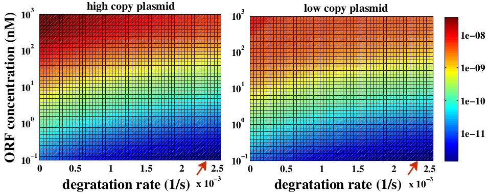
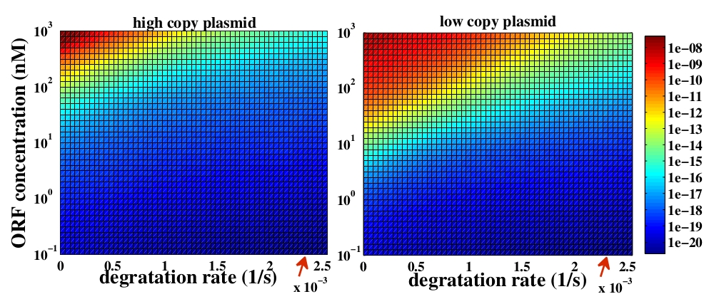
The variable we are interested in optimizing is the concentration of Plug&Play plasmids with the inserted ORF. This variable is presented as a function of the degradation rate k_d and ORF concentration in figure 3 and 4, for CRE and FLP, respectively. The value of RNA degradation rate is indicated by a red arrow.

For CRE recombinase, linear DNA degradation do not play a fundamental role in our system and it can even be disregarded, figure 3. This may occur because the circularization of linear DNA by recombinases is faster than the degradation of it. For FLP, however, linear DNA degradation is an important effect and must be taken in account, figure 4. This occurs because the association of the first and second monomers for CRE is significantly higher than for FLP.

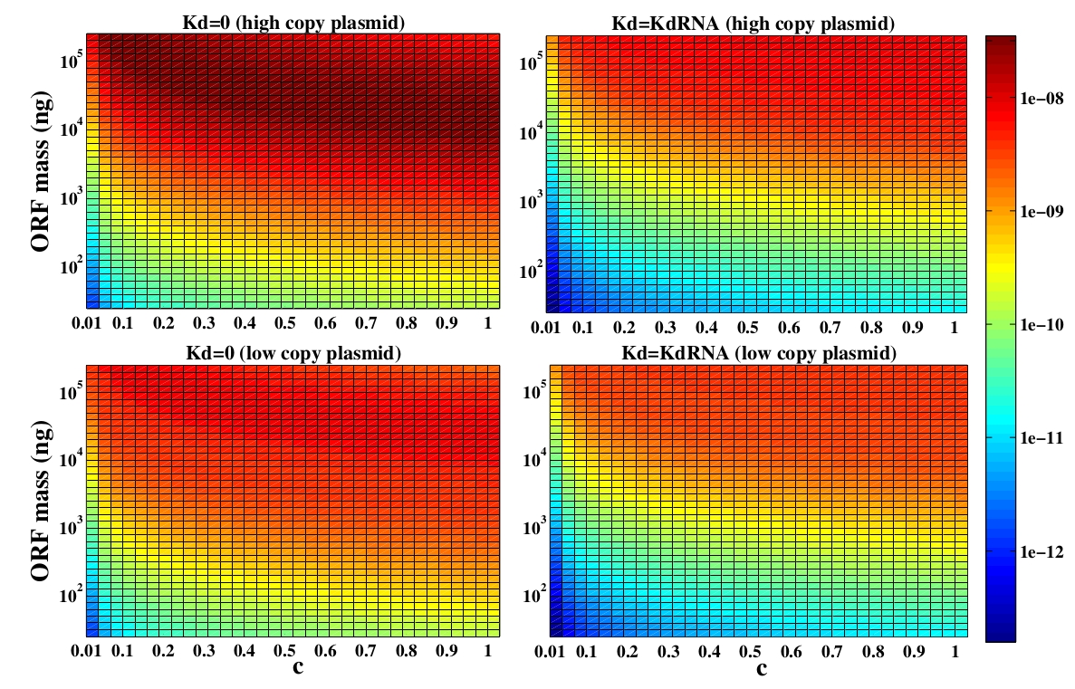
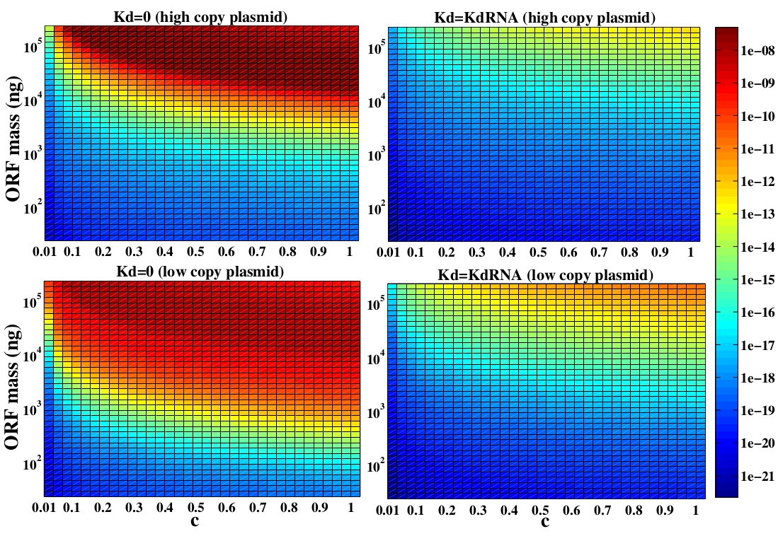
In the following analysis we evaluated the concentration of plasmids with the inserted ORF as a function of the DNA mass in the solution during eletroporation and the variable c (the fraction of ORF concentration that enters in the bacteria), Figs 5 and 6. We are interested in concentrations of Plug&Play plasmids with the ORF inserted higher than 1 $nM$ which means that, in average, there will be at least one plasmid with the ORF in the bacteria, represented by the red region on the Figs. 5 and 6. According to our results an amount of 10000 $ng$ of DNA might be satisfactory when using CRE. Nevertheless, when using FLP this amount might not be enough and the amount needed is highly dependent of the linear DNA degradation rate.

One possible strategy to improve the recombination without increasing this amount of DNA is to reduce the volume of the solution before eletroporation, which increase the ORF concentration in the solution. Values lower than 10000 $ng$ of DNA may also be satisfactory since the ORF has a antibiotics resistance gene and once the ORF had been inserted the bacteria tend to keep and replicate the plasmid.

Discussion

In order to identify differences between FLP and CRE, we compared the two enzymes using two analyses. Our results point to an obvious choice for the CRE-lox recombination system since it is less affected by DNA degradation and improves the insertion of the ORF compared with FLP-FRT system.

In our model we have considered all lox sites as loxP. However, there are mutated loxP and a combination of them can improve the insertion of the target gene (ORF) [4]. We have chosen to use lox66 and lox71 in our experimental design. Nevertheless, we did not introduce the lox66 and lox71 in the model for two main reasons: there are no references about the values of rate constants for altered loxP and we prefer to keep the simplicity and clarity of the model. In order to take these variables in consideration, it would be necessary to use more equations and extra hypothesis.

Although we did not consider the mutated loxP, we have some considerations about it. The insertion reaction is favored over the excision reaction by roughly fivefold using mutated recombination, when using CRE recombinases [4]. This occurs because the double mutated loxP has a very low affinity for the CRE monomers. So, an intuitive conclusion is that the combination we chose may optimize the insertion of the ORF in the Plug&Play plasmid. Nevertheless, this conclusion could be false because the altered loxP demands more time in the circularization step since it has a lower association constant for CRE recombinase. This extra amount of time could be such that the degradation of linear DNA plays a fundamental role in the process. However, as it is illustrated in Fig. 3, in the case of CRE recombinases, the degradation of linear DNA is not a fundamental variable and it may not interfere. Because of that, we may conclude that the combination of mutated loxP must optimize the amount of ORF inserted in the plasmid.

Appendix

Equations

\begin{align} &\frac{d}{dt}[S] = k_{-1}[S_{a}] - [S](k_{1}[M] + k_{d}) \nonumber \\ &\frac{d}{dt}[S_{a}] = k_{1}[S][M] + k_{-1}[S_{aa}] + k_{-2}[S_{ab}] - [S_{a}]( k_{1}[M] + k_{-1} + k_{2}[M] + k_{d} ) \nonumber \\ &\frac{d}{dt}[S_{aa}] = k_{1}[S_{a}][M] + k_{-2}[S_{3}] - [S_{aa}](k_{2}[M] + k_{-1} + k_{d}) \nonumber \\ &\frac{d}{dt}[S_{ab}] = k_{2}[S_{a}][M] + k_{-1}[S_{3}] - [S_{ab}](k_{-2} + k_{1}[M] + k_{d}) \nonumber \\ &\frac{d}{dt}[S_{3}] = k_{1}[S_{ab}][M] + k_{2}[S_{aa}][M] + k_{-2}[S_{4}] - [S_{3}](k_{-1} + k_{-2} + k_{2}[M] + k_{d}) \nonumber \\ &\frac{d}{dt}[S_{4}] = k_{2}[S_{3}][M] + k_{-34}[I_c] - [S_{4}](k_{-2} + k_{34} + k_{d}) \nonumber \\ &\frac{d}{dt}[I_c] = k_{34}[S_{4}] + k_{-5}[L_{2}][C_{2}] - [I_c](k_{-34} + k_{-5}) \nonumber \\ &\frac{d}{dt}[C_{2}] = k_{5}[I_c] + k_{2}[C_{1}][M] - [C_{2}](k_{-5}[P_{2}] + k_{-2}) \nonumber \\ &\frac{d}{dt}[C_{1}] = k_{1}[C][M] + k_{-2}[C_{2}] - [C_{1}](k_{-1} + k_{2}[M]) \nonumber \\ &\frac{d}{dt}[C] = k_{-1}[C_{1}] - k_{1}[M][C] \nonumber \\ &\frac{d}{dt}[L_{2}] = k_{5}[I_c] + k_{2}[L_{1}][M] - [L_{2}](k_{-5}[C_{2}] + k_{-2} + k_{d}) \\ &\frac{d}{dt}[L_{1}] = k_{1}[L][M] + k_{-2}[L_{2}] - [L_{1}](k_{-1}+ k_{2}[M] + k_{d}) \nonumber \\ &\frac{d}{dt}[L] = k_{-1}[L_{1}] - [L](k_{1}[M] + k_{d}) \nonumber \\ &\frac{d}{dt}[P] = k_{-1}[P_{1}] - k_{1}[M][P] \nonumber \\ &\frac{d}{dt}[P_{1}] = k_{1}[P][M] + k_{-2}[P_{2}] - [P_{1}](k_{-1} + k_{2}[M]) \nonumber \\ &\frac{d}{dt}[P_{2}] = k_{5}[I] + k_{2}[P_{1}][M] - [P_{2}](k_{-5}[C_{2}] + k_{-2}) \nonumber \\ &\frac{d}{dt}[I] = k_{34}[M_{4}] + k_{-5}[P_{2}][C_{2}] - [I](k_{-34} + k_{5}) \nonumber \\ &\frac{d}{dt}[E_{4}] = k_{-34}[I] + k_{2}[E_{3}][M] - [E_{4}](k_{34}+ k_{-2}) \nonumber \\ &\frac{d}{dt}[E_{3}] = k_{-2}[E_{4}] + k_{2}[E_{aa}][M] + k_{1}[E_{ab}][M] - [E_{3}](k_{2}[M] + k_{-2} + k_{-1}) \nonumber \\ &\frac{d}{dt}[E_{aa}]= k_{-2}[E_{3}] + k_{1}[E_{a}][M] - [E_{aa}](k_{2}[M] + k_{-1}) \nonumber \\ &\frac{d}{dt}[E_{ab}]= k_{-1}[E_{3}] + k_{2}[E_{a}][M] - [E_{ab}](k_{1}[M] + k_{-2}) \nonumber \\ &\frac{d}{dt}[E_{a}] = k_{-1}[E_{aa}] + k_{-2}[E_{ab}] + k_{1}[E][M] - [E_{a}](k_{1}[M] + k_{2}[M] + k_{-1}) \nonumber \\ &\frac{d}{dt}[E] = k_{-1}[E_{a}] - k_{1}[M][E] \nonumber \end{align}

References

[1] L. Ringrose, V. Lounnas, L. Ehrlich, F. Buchholz, R. Wade and A.F. Stewart Comparative kinetic analysis of FLP and cre recombinases: mathematical models for DNA binding and recombination. Journal of Molecular Biology (1998) 284, 363–384

[2] http://bionumbers.hms.harvard.edu/

[3] http://partsregistry.org/

[4] Zuwen Zhang and Beat Lutz. Cre recombinase-mediated inversion using lox66 and lox71: method to introduce conditional point mutations into the CREB-binding protein. Nucl. Acids Res. (2002) 30 (17): e90.