Team:Colombia/Modeling/Ecological Model
From 2012.igem.org
(→Graphical Model) |
(→Implementation Model scripting check) |
||
| (59 intermediate revisions not shown) | |||
| Line 6: | Line 6: | ||
{{https://2012.igem.org/User:Tabima}} | {{https://2012.igem.org/User:Tabima}} | ||
| - | = | + | <div class="right_box"> |
| - | + | =Implementation Model= | |
'''General objective''' | '''General objective''' | ||
| - | To generate a computational model that simulates the most relevant | + | To generate a computational model that simulates the most relevant relationships between our engineered system and the plant pathogens inside the appropriate habitat for the Rust control. |
'''Specific Objectives''' | '''Specific Objectives''' | ||
| - | - To limit the multifactorial ecological problem in a way that a simple mathematical model may be proposed. Such model should be able to answer relevant questions regarding the | + | - To limit the multifactorial ecological problem in a way that a simple mathematical model may be proposed. Such model should be able to answer relevant questions regarding the implementation method. |
| - | - To find the populational proportions between our organism | + | - To find the populational proportions between our organism and the plant pathogens that optimize our biological control. |
- To generate hypotheses for future experimental confirmations. | - To generate hypotheses for future experimental confirmations. | ||
| - | == | + | ==Biological Panorama== |
| - | [[ | + | Coffee Rust dispersion is based on the generation of [http://botanydictionary.org/uredospore.html uredospores]. These are dispersed by wind and water predominantly, as well as by active animal or human dispersion. These spores require about 24 to 48 hours of free continuous humidity, so the infection process usually occur only during rainy seasons. The fungus grows as a [http://en.wikipedia.org/wiki/Mycelium mycelium] on the leaves of the plant, and the generation of new spores takes about 10 to 14 days. Since leaves drop prematurely, this effectively removes important quantities of epidemic potential inoculum; nevertheless, a few green leaves will survive through the dry season. Dry uredospores may live for about 6 weeks. In this way, there is always a viable inoculum capable of infecting new leaves ath the beginning of the next rainy season. |
| - | + | In this year's iGEM, our main goal is to significatively reduce the mycelial form of the fungus in order to control inocula from a season to the next. The way this works is by spraying bacteria on top of the leaves of the plants, however, the amount and concentration of bacteria are not known. Thanks to a [https://2012.igem.org/Team:Colombia/Project/Experiments/Our_Design population control system by toxin-antitoxin modules], a small fraction (near 15%) of the bacterial population will live in a persistant state. Persister cells have very low metabolic rates. Non-persister active cells, even though more sensitive to environmental hazards, readily detect fungal infections. If a determined chitin profile (based on our [https://2012.igem.org/Team:Colombia/Modeling/Paramterers molecular mathematical models]) is detected, active bacteria are stimulated in a way that they are capable of secreting a plant hormone to induce its natural defense responses. | |
| - | ''We | + | ==Mathematical Model Description== |
| + | |||
| + | Let's begin with the expected dynamics for the inoculated bacteria in absence of a fungal infection (''R'' variable). An initial number of bacteria (''B'' variable) are sprayed on the leaf. As mentioned earlier, these may be in a persistant (''I'' variable) or active (''A^--'' variable) state in a 15:85 ratio. By assuming persistence as a static metabolic state, persister death rate is neglected. On the other hand, active bacteria die with a given rate (''delta_A'' parameter per active bacterium). However, these populations are maintained through a dynamic equilibrium with a persistance transition rate (''gamma_1'' parameter per active bacterium), and another one in the reverse direction (''alpha(R)'' parameter per persister bacterium). The ''alpha(R)'' parameter should, in principle, have a term independant of ''R'' in order to maintain the described equilibrium. If this were not true, ''A^-'' would have no population inputs and would decay to zero in steady state. | ||
| + | |||
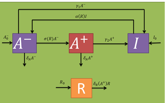
| + | In the presence of fungi, cells should wake up more often (which should be included in the ''alpha(R)'' parameter). Additionally, the ''A^--'' population should generate a stimulated cell population (''A^+'' variable) at a certain rate (''sigma(R)'' parameter per inactive bacterium). Stimulated bacteria are capable of producing salycilic acid, a plant hormone that induces plant defense mechanisms that should decrease fungal populations at a given rate (''delta_R(A^+)'' per fungus). The only fungi relevant to our model are those who already germinated from the uredospores and are infecting the plant (i.e., that are in a mycelial form). Taking this into account, their random removal and natural death rates are neglected. In the same fashion as with the active cell population, stimulated once are capable of returning to a persister state with a certain rate (''gamma_2'' parameter per stimulated bacterium) and also eventually die at a given rate (which we approximated to be comparable to the active one's). Persister state stimulating toxins act at a intercellular level, so cell cross-activation/inactivation phenomena are discarded. The following schematic represents the expected population dynamics for this model for a single infection cycle. Subsequent cycles should work in a similar fashion, where the next cycle's inputs are the previous cycle's outputs. | ||
| + | |||
| + | [[File:ecomoda.png|thumb|center|500px|Figure 1. Expected population dynamics ]] | ||
| + | |||
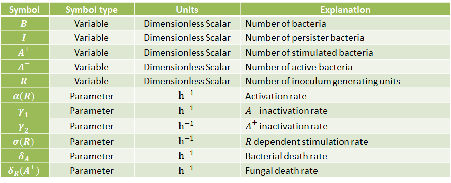
| + | The following table indicates the different parameters and variables of our system, together with its units and explanation. | ||
| + | |||
| + | [[File:ecotabla.png|center|thumb|700px|Table 1. Parameters and variables of this system ]] | ||
| + | |||
| + | === Differential Equations === | ||
| + | |||
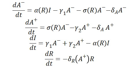
| + | From the schematic above the following ordinary differential equations were constructed: | ||
| + | |||
| + | [[File:ecodif.png|center]] | ||
| + | |||
| + | As well as the following initial conditions: | ||
| + | |||
| + | [[File:ecocondin.png|center]] | ||
| + | |||
| + | === Inferences from the Molecular Mathematical Model=== | ||
| + | |||
| + | First of all we had to find our parameters' values, as well as define some of those more thoroughly. | ||
| + | |||
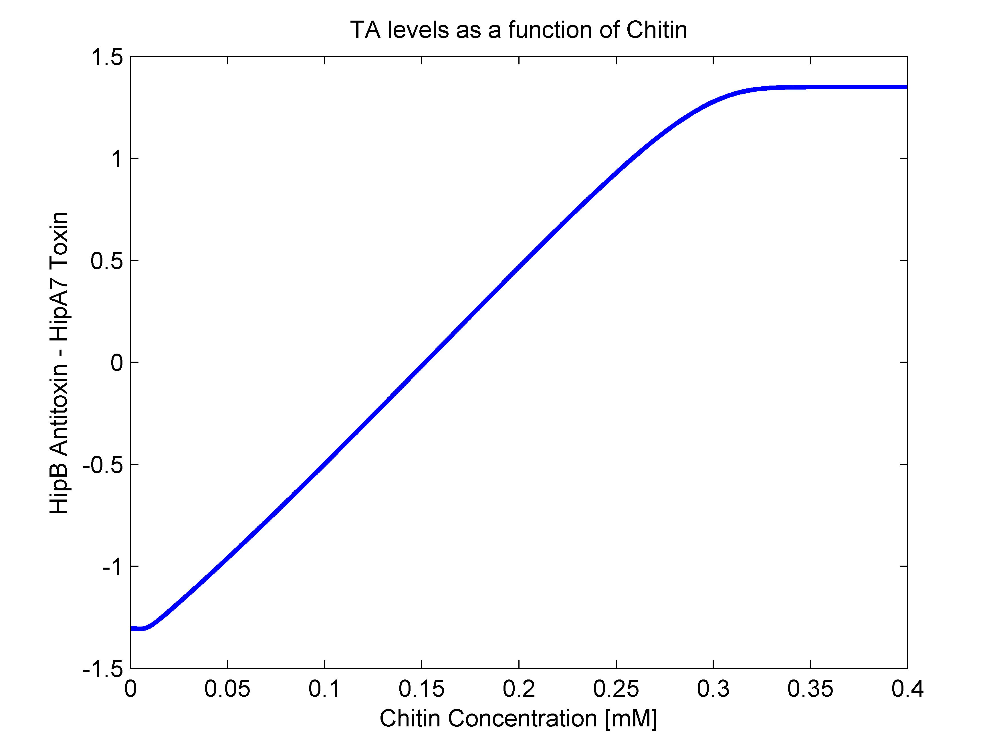
| + | - ''alpha(R)'': As mentioned earlier, this parameter should have both ''R'' dependent and independent terms. The independent term was searched for in literature, where we found it to be 0.1 h^-1 (Balaban et al, 2004). For the ''R'' dependent term, we thought of two possibilities. The first one that it may be aproximated as a line in the form of ''beta*R'', and the second one as a heaviside function (step function). In order to answer this, we went back to our original mathematical molecular model and plotted chitin concentration against the difference between toxin and antitoxin concentrations. This should give us an idea of the shape of the function we are looking for. The following figure shows how ''alpha(R)'' heavily resembles a line, so we went for the linear option (''beta'' slope = 0.103562). | ||
| + | |||
| + | [[File:figuraalfa.png|center|500px|thumb|Figure 2. Toxin-Antitoxin levels as a function of chitin concentration ]] | ||
| + | |||
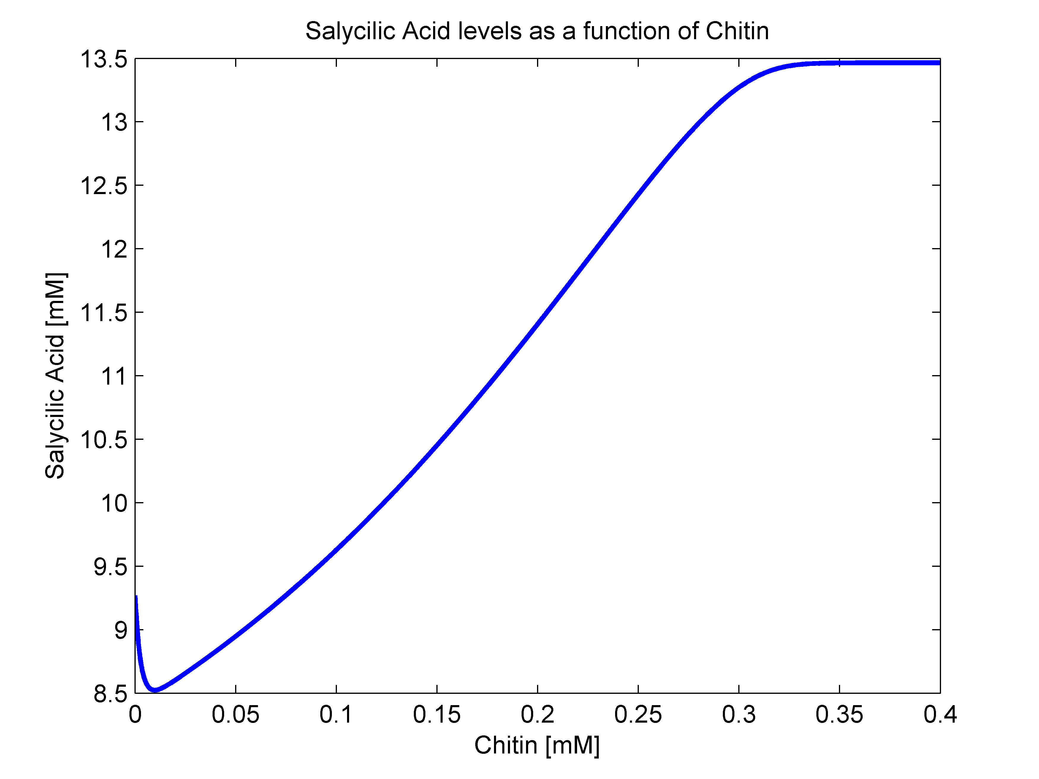
| + | - ''sigma(R)'': Because of the way that we defined our bacterial states, there is no way that there are intermediate states between our activated and stimulated populations. With this in mindo we decided that the stimulation transition state was to be described with a heaviside step function. This function's value is zero until a certain criterion is met. In our case, that is that the R value surpasses a given threshold. Since we were not able to measure how much chitin in a Coffee Rust sample, we decided to transform our ''R'' function to a chitin function. This should not be a problem since their relationship should behave linearly. As a way to define an ''Rnot'', that is, the chitin threshold for successful stimulation, we went back to our molecular mathematical model and plotted chitin concentration against salycilic acid. The chitin concentration that gave us half the maximum production of salycilic acid would be the value chosen for ''Rnot''. We successfully estimated ''Rnot'' = 0.19124 mM from the following figure. | ||
| + | |||
| + | [[File:figurarnot.png|center|500px|thumb|Figure 3. Salycilic acid level as a function of chitin concentration]] | ||
| + | |||
| + | - ''gamma_1'': We looked for persistence transition rates in the literature and found that ''gamma_1'' = 1.2e-6 h^-1(Balaban et al, 2004). | ||
| + | |||
| + | - ''gamma_2'': Since we haven't measured our own final stimulated bacteria persistence transition rate, we estimated it to be about 5% of ''gamma_1''. We have engineered our system in such a way that ''gamma_1'' should be a lot greater that ''gamma_2'', so 5% is actually an overestimation. | ||
| + | |||
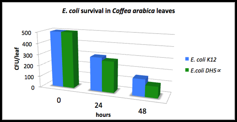
| + | - ''delta_A'': [https://2011.igem.org/Team:Colombia Last year's Colombia iGEM team] measured the ''Escherichia coli'' DH5alpha and ''E. coli'' K12 survival on top of the coffee plants for 48 hours (measurements not in wiki). They inoculated a total of 500 UFC/leaf at the starting time and observed the remaining UFC/leaf 24 aand 48 hours later. The following graph shows their results. We fitted the average of both columns into an exponential distribution and estimated ''delta_A'' = 0.035 h^-1. | ||
| + | |||
| + | [[File:leafcount.png|center|500px|thumb|Figure 4. E. coli survival in coffee leaves]] | ||
| + | |||
| + | - ''delta_R(A^+)'': Since the plant's response is the disposal of the whole leaf, and we are currently modeling a single leaf, we decided to use an inverse heaviside step function for this parameter. In words, once the stimulated bacterial cell population reaches a certain threshold, all living fungi will die off the leaf, because the Coffee Rust needs its host to be alive in order to live. We named this threshold ''Anot''. Ideally, we need to estimate, given our current molecular constructions, how much Salycilic Acid is produced per stimulated cell in order to determine ''Anot'', as well as what is the minumum amount of salycilic acid the plant needs to optimize its defense response. Unfortunately, such measurements have not been made yet. In the next sections we check that our model works correctly and discuss a method to calculate the optimal amount of bacteria to spray onto the leaf for optimal implementation. | ||
| + | |||
| + | === Implementation Model scripting check === | ||
| + | |||
| + | As mentioned earlier, we are one parameter short (''Anot'') to be able to objectively minimize the number of bacteria needed to be sprayed onto the leaves for a successful biological control. However, we guesstimated both ''B'' and ''Anot'' in order to see how our model's results should look like. We wrote the following two codes that solve our differential equations: | ||
| + | |||
| + | % Differential Equations | ||
| + | |||
| + | function output = ode(dt, v) | ||
| + | |||
| + | %% Biological Parameters | ||
| + | |||
| + | alpha = 0.1; % basal wake up rate Balaban et al [1/h] | ||
| + | beta = 0.103562; % chitin induced wake up rate | ||
| + | Rnot = 0.19124; % The amount of chitin necessary to activate 'a' | ||
| + | gamma1 = 1.2e-6; % 'a'sleep rate [1/h] | ||
| + | gamma2 = 0.05*gamma1; % 'A' sleep rate [1/h] | ||
| + | deltaA = 0.035; % E.coli death rate in leaves [1/h] | ||
| + | Anot = 3500; % 'A' cells required for effective plant defense induction | ||
| + | |||
| + | %% Differential Equations | ||
| + | |||
| + | I = v(1); % Import 'I' cell number | ||
| + | a = v(2); % Import 'a' cell number | ||
| + | A = v(3); % Import 'A' cell number | ||
| + | R = v(4); % Import 'R' chitin concentration | ||
| + | |||
| + | dI = gamma1*a + gamma2*A - (alpha + beta*R)*I; | ||
| + | % 'I' cell ODE | ||
| + | |||
| + | da = (alpha + beta*R)*I - gamma1*a - heaviside(R - Rnot)*a - deltaA*a; | ||
| + | % 'a' cell ODE | ||
| + | |||
| + | dA = heaviside(R - Rnot)*a - gamma2*A - deltaA*A; | ||
| + | % 'A' cell ODE | ||
| + | |||
| + | if A < Anot % Plant Defense check | ||
| + | dR = 0; | ||
| + | else dR = -1000*R; | ||
| + | end | ||
| + | |||
| + | output1(1) = dI; | ||
| + | output1(2) = da; | ||
| + | output1(3) = dA; | ||
| + | output1(4) = dR; | ||
| + | |||
| + | output = output1'; | ||
| + | |||
| + | end | ||
| + | |||
| + | %Solver Implementation model | ||
| + | |||
| + | clear; clc; close all; | ||
| + | |||
| + | %% Biological Parameters | ||
| + | |||
| + | B = 5e3; % Number of initial bacteria | ||
| + | a0 = 0.85*B; % Estimated basal 'a' cell proportion | ||
| + | I0 = 0.15*B; % Estimated basal persister proportion | ||
| + | R0 = 0.2; % Successful Pestbuster response chitin concentration | ||
| + | A0 = 0; % Initial activated 'a' cells | ||
| + | |||
| + | %% Solver Parameters | ||
| + | |||
| + | h = 50; % Maximum Time | ||
| + | |||
| + | m = 0.01; % Time step [h] | ||
| + | |||
| + | t = 0:m:h; % Time Vector | ||
| + | |||
| + | l = (0:m:h)'; % Column time vector | ||
| + | |||
| + | x = zeros(length(l), 4); % Result matriz initialization | ||
| + | % Columns represent I, a, A, and R quantities | ||
| + | % Rows represent each time step | ||
| + | |||
| + | x(1,:) = [I0 a0 A0 R0]; % Initial conditions | ||
| + | |||
| + | %% Differential equation 4th order Runge-Kutta method (RK4) | ||
| + | |||
| + | for k = 1:length(l) - 1 | ||
| + | |||
| + | xk = x(k,:); % Extract most recent population numbers | ||
| + | |||
| + | k1 = ode(l(k),xk); % First RK4 slope | ||
| + | k2 = ode(l(k) + m/2,xk + (m/2*k1)'); % Second RK4 slope | ||
| + | k3 = ode(l(k) + m/2,xk + (m/2*k2)'); % Third RK4 slope | ||
| + | k4 = ode(l(k) + m,xk + (m*k3)'); % Fourth RK4 slope | ||
| + | |||
| + | xk1 = xk + m/6*(k1 + 2*k2 + 2*k3 + k4)'; | ||
| + | % New population numbers calculation | ||
| + | |||
| + | xk2 = zeros(1,length(xk1)); | ||
| + | % Row vector initialization | ||
| + | |||
| + | for p = 1:length(xk1) | ||
| + | |||
| + | if(xk1(p) < 0.00000001) % Tolerance check | ||
| + | |||
| + | xk2(p) = 0; | ||
| + | else | ||
| + | xk2(p) = xk1(p); | ||
| + | end | ||
| + | end | ||
| + | |||
| + | x(k + 1,:) = xk2(:); | ||
| + | end | ||
| + | |||
| + | %% Plots | ||
| + | |||
| + | I = x(:,1); % 'I' cell vector | ||
| + | a = x(:,2); % 'a' cell vector | ||
| + | A = x(:,3); % 'A' cell vector | ||
| + | R = x(:,4); % Chitin vector | ||
| + | |||
| + | figure | ||
| + | subplot(2,2,1) | ||
| + | P1 = plot(l,I); | ||
| + | set(P1,'LineWidth',2) | ||
| + | title('Persister Cells [I]') | ||
| + | xlabel('Time [h]') | ||
| + | ylabel('Persister Cell Number') | ||
| + | |||
| + | subplot(2,2,2) | ||
| + | P2 = plot(l,a); | ||
| + | set(P2,'LineWidth',2) | ||
| + | title('Unstimulated Woken up Cells [a]') | ||
| + | xlabel('Time [h]') | ||
| + | ylabel('Unsitmulated Woken up Cell Number') | ||
| + | |||
| + | subplot(2,2,3) | ||
| + | P3 = plot(l,A); | ||
| + | set(P3,'LineWidth',2) | ||
| + | title('Activated Cells [A]') | ||
| + | xlabel('Time [h]') | ||
| + | ylabel('Activated Cell Number') | ||
| + | |||
| + | subplot(2,2,4) | ||
| + | P4 = plot(l,R); | ||
| + | set(P4,'LineWidth',2) | ||
| + | title('Rust fungi [R]') | ||
| + | xlabel('Time [h]') | ||
| + | ylabel('Leaf Chitin Concentration') | ||
| + | |||
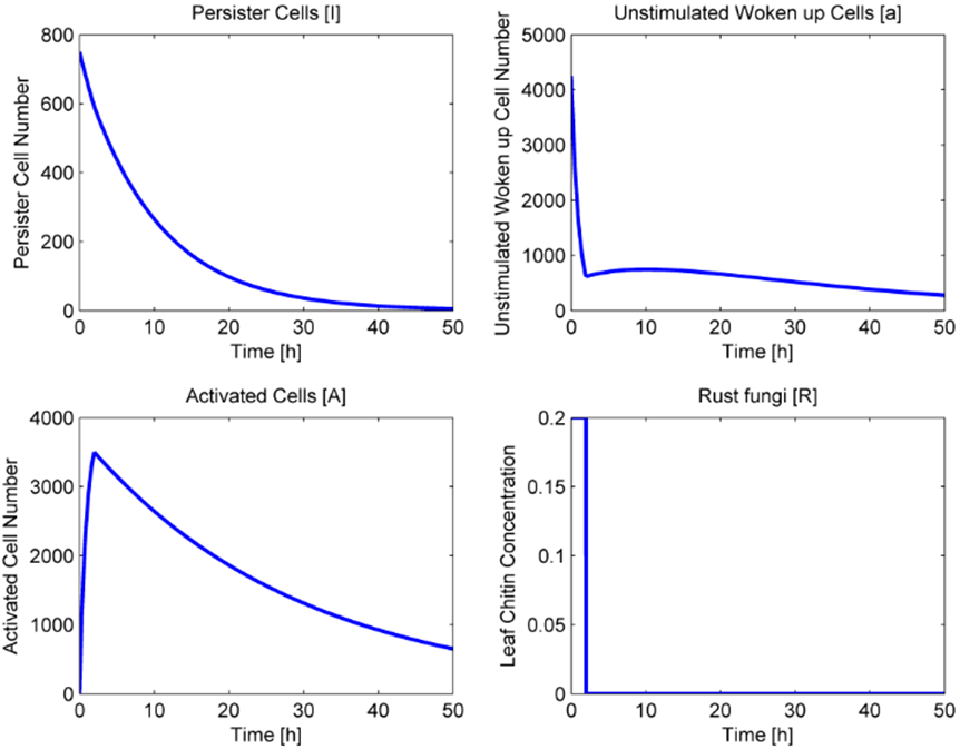
| + | If you run these codes you get the following plots: | ||
| + | |||
| + | [[File:elcheck.jpg|center|700px|thumb|Figure 5. Model check results]] | ||
| + | |||
| + | The model works as expected. When chitin (fungi) is present, the persister and activated cell count decay to give rise to stimulated cells. Once these surpass the ''Anot'' 3500 threshold, the leaf drops and the fungi count goes to zero. The activated cell plot presents two distinct distributions, a first one of exponential decay (when R is present)and a second one (when the fungus dies). The second one shows an initial rise to steady state and then another decay due to cell death. | ||
| + | |||
| + | === Model Usage === | ||
| + | |||
| + | While we are waiting for experimental results to be able to infer the minimum Bacterial numbers to spray into the plant, we have deviced a method to calculate this number once we know ''Anot''. Using the above code, we can probe for different ''Anot'' values and check the minimum ''B'' number that effectively eliminates fungi. We then, plot valid ''Anot'' against their minimum ''B'' values. In this way, we may fit a distribution to this data and then calulate the nomber of bacteria we need for the experimentally obtained ''Anot''. | ||
| + | |||
| + | ==References== | ||
| + | #Balaban, N. Q., Merrin, J., Chait, R., Kowalik, L., & Leibler, S. (2004). Bacterial persistence as a phenotypic switch. Science (New York, N.Y.), 305(5690), 1622–5. doi:10.1126/science.1099390 | ||
Latest revision as of 03:59, 27 October 2012
Template:Https://2012.igem.org/User:Tabima
Contents |
Implementation Model
General objective
To generate a computational model that simulates the most relevant relationships between our engineered system and the plant pathogens inside the appropriate habitat for the Rust control.
Specific Objectives
- To limit the multifactorial ecological problem in a way that a simple mathematical model may be proposed. Such model should be able to answer relevant questions regarding the implementation method.
- To find the populational proportions between our organism and the plant pathogens that optimize our biological control.
- To generate hypotheses for future experimental confirmations.
Biological Panorama
Coffee Rust dispersion is based on the generation of [http://botanydictionary.org/uredospore.html uredospores]. These are dispersed by wind and water predominantly, as well as by active animal or human dispersion. These spores require about 24 to 48 hours of free continuous humidity, so the infection process usually occur only during rainy seasons. The fungus grows as a [http://en.wikipedia.org/wiki/Mycelium mycelium] on the leaves of the plant, and the generation of new spores takes about 10 to 14 days. Since leaves drop prematurely, this effectively removes important quantities of epidemic potential inoculum; nevertheless, a few green leaves will survive through the dry season. Dry uredospores may live for about 6 weeks. In this way, there is always a viable inoculum capable of infecting new leaves ath the beginning of the next rainy season.
In this year's iGEM, our main goal is to significatively reduce the mycelial form of the fungus in order to control inocula from a season to the next. The way this works is by spraying bacteria on top of the leaves of the plants, however, the amount and concentration of bacteria are not known. Thanks to a population control system by toxin-antitoxin modules, a small fraction (near 15%) of the bacterial population will live in a persistant state. Persister cells have very low metabolic rates. Non-persister active cells, even though more sensitive to environmental hazards, readily detect fungal infections. If a determined chitin profile (based on our molecular mathematical models) is detected, active bacteria are stimulated in a way that they are capable of secreting a plant hormone to induce its natural defense responses.
Mathematical Model Description
Let's begin with the expected dynamics for the inoculated bacteria in absence of a fungal infection (R variable). An initial number of bacteria (B variable) are sprayed on the leaf. As mentioned earlier, these may be in a persistant (I variable) or active (A^-- variable) state in a 15:85 ratio. By assuming persistence as a static metabolic state, persister death rate is neglected. On the other hand, active bacteria die with a given rate (delta_A parameter per active bacterium). However, these populations are maintained through a dynamic equilibrium with a persistance transition rate (gamma_1 parameter per active bacterium), and another one in the reverse direction (alpha(R) parameter per persister bacterium). The alpha(R) parameter should, in principle, have a term independant of R in order to maintain the described equilibrium. If this were not true, A^- would have no population inputs and would decay to zero in steady state.
In the presence of fungi, cells should wake up more often (which should be included in the alpha(R) parameter). Additionally, the A^-- population should generate a stimulated cell population (A^+ variable) at a certain rate (sigma(R) parameter per inactive bacterium). Stimulated bacteria are capable of producing salycilic acid, a plant hormone that induces plant defense mechanisms that should decrease fungal populations at a given rate (delta_R(A^+) per fungus). The only fungi relevant to our model are those who already germinated from the uredospores and are infecting the plant (i.e., that are in a mycelial form). Taking this into account, their random removal and natural death rates are neglected. In the same fashion as with the active cell population, stimulated once are capable of returning to a persister state with a certain rate (gamma_2 parameter per stimulated bacterium) and also eventually die at a given rate (which we approximated to be comparable to the active one's). Persister state stimulating toxins act at a intercellular level, so cell cross-activation/inactivation phenomena are discarded. The following schematic represents the expected population dynamics for this model for a single infection cycle. Subsequent cycles should work in a similar fashion, where the next cycle's inputs are the previous cycle's outputs.
The following table indicates the different parameters and variables of our system, together with its units and explanation.
Differential Equations
From the schematic above the following ordinary differential equations were constructed:
As well as the following initial conditions:
Inferences from the Molecular Mathematical Model
First of all we had to find our parameters' values, as well as define some of those more thoroughly.
- alpha(R): As mentioned earlier, this parameter should have both R dependent and independent terms. The independent term was searched for in literature, where we found it to be 0.1 h^-1 (Balaban et al, 2004). For the R dependent term, we thought of two possibilities. The first one that it may be aproximated as a line in the form of beta*R, and the second one as a heaviside function (step function). In order to answer this, we went back to our original mathematical molecular model and plotted chitin concentration against the difference between toxin and antitoxin concentrations. This should give us an idea of the shape of the function we are looking for. The following figure shows how alpha(R) heavily resembles a line, so we went for the linear option (beta slope = 0.103562).
- sigma(R): Because of the way that we defined our bacterial states, there is no way that there are intermediate states between our activated and stimulated populations. With this in mindo we decided that the stimulation transition state was to be described with a heaviside step function. This function's value is zero until a certain criterion is met. In our case, that is that the R value surpasses a given threshold. Since we were not able to measure how much chitin in a Coffee Rust sample, we decided to transform our R function to a chitin function. This should not be a problem since their relationship should behave linearly. As a way to define an Rnot, that is, the chitin threshold for successful stimulation, we went back to our molecular mathematical model and plotted chitin concentration against salycilic acid. The chitin concentration that gave us half the maximum production of salycilic acid would be the value chosen for Rnot. We successfully estimated Rnot = 0.19124 mM from the following figure.
- gamma_1: We looked for persistence transition rates in the literature and found that gamma_1 = 1.2e-6 h^-1(Balaban et al, 2004).
- gamma_2: Since we haven't measured our own final stimulated bacteria persistence transition rate, we estimated it to be about 5% of gamma_1. We have engineered our system in such a way that gamma_1 should be a lot greater that gamma_2, so 5% is actually an overestimation.
- delta_A: Last year's Colombia iGEM team measured the Escherichia coli DH5alpha and E. coli K12 survival on top of the coffee plants for 48 hours (measurements not in wiki). They inoculated a total of 500 UFC/leaf at the starting time and observed the remaining UFC/leaf 24 aand 48 hours later. The following graph shows their results. We fitted the average of both columns into an exponential distribution and estimated delta_A = 0.035 h^-1.
- delta_R(A^+): Since the plant's response is the disposal of the whole leaf, and we are currently modeling a single leaf, we decided to use an inverse heaviside step function for this parameter. In words, once the stimulated bacterial cell population reaches a certain threshold, all living fungi will die off the leaf, because the Coffee Rust needs its host to be alive in order to live. We named this threshold Anot. Ideally, we need to estimate, given our current molecular constructions, how much Salycilic Acid is produced per stimulated cell in order to determine Anot, as well as what is the minumum amount of salycilic acid the plant needs to optimize its defense response. Unfortunately, such measurements have not been made yet. In the next sections we check that our model works correctly and discuss a method to calculate the optimal amount of bacteria to spray onto the leaf for optimal implementation.
Implementation Model scripting check
As mentioned earlier, we are one parameter short (Anot) to be able to objectively minimize the number of bacteria needed to be sprayed onto the leaves for a successful biological control. However, we guesstimated both B and Anot in order to see how our model's results should look like. We wrote the following two codes that solve our differential equations:
% Differential Equations

function output = ode(dt, v)

%% Biological Parameters

alpha = 0.1; % basal wake up rate Balaban et al [1/h]
beta = 0.103562; % chitin induced wake up rate
Rnot = 0.19124; % The amount of chitin necessary to activate 'a'
gamma1 = 1.2e-6; % 'a'sleep rate [1/h]
gamma2 = 0.05*gamma1; % 'A' sleep rate [1/h]
deltaA = 0.035; % E.coli death rate in leaves [1/h]
Anot = 3500; % 'A' cells required for effective plant defense induction

%% Differential Equations

I = v(1); % Import 'I' cell number
a = v(2); % Import 'a' cell number
A = v(3); % Import 'A' cell number
R = v(4); % Import 'R' chitin concentration

dI = gamma1*a + gamma2*A - (alpha + beta*R)*I;
% 'I' cell ODE

da = (alpha + beta*R)*I - gamma1*a - heaviside(R - Rnot)*a - deltaA*a;
% 'a' cell ODE

dA = heaviside(R - Rnot)*a - gamma2*A - deltaA*A;
% 'A' cell ODE

if A < Anot % Plant Defense check
    dR = 0;
else dR = -1000*R;
end

output1(1) = dI;
output1(2) = da;
output1(3) = dA;
output1(4) = dR;

output = output1';

end
%Solver Implementation model

clear; clc; close all;

%% Biological Parameters

B = 5e3; % Number of initial bacteria
a0 = 0.85*B; % Estimated basal 'a' cell proportion
I0 = 0.15*B; % Estimated basal persister proportion
R0 = 0.2; % Successful Pestbuster response chitin concentration
A0 = 0; % Initial activated 'a' cells

%% Solver Parameters

h = 50; % Maximum Time

m = 0.01; % Time step [h]

t = 0:m:h; % Time Vector

l = (0:m:h)'; % Column time vector

x = zeros(length(l), 4); % Result matriz initialization
% Columns represent I, a, A, and R quantities
% Rows represent each time step

x(1,:) = [I0 a0 A0 R0]; % Initial conditions

%% Differential equation 4th order Runge-Kutta method (RK4)

for k = 1:length(l) - 1

   xk = x(k,:); % Extract most recent population numbers

   k1 = ode(l(k),xk); % First RK4 slope
   k2 = ode(l(k) + m/2,xk + (m/2*k1)'); % Second RK4 slope
   k3 = ode(l(k) + m/2,xk + (m/2*k2)'); % Third RK4 slope
   k4 = ode(l(k) + m,xk + (m*k3)'); % Fourth RK4 slope

   xk1 = xk + m/6*(k1 + 2*k2 + 2*k3 + k4)';
   % New population numbers calculation

   xk2 = zeros(1,length(xk1));
   % Row vector initialization

   for p = 1:length(xk1)

       if(xk1(p) < 0.00000001) % Tolerance check

           xk2(p) = 0;
       else
           xk2(p) = xk1(p);
       end
   end

   x(k + 1,:) = xk2(:);
end

%% Plots

I = x(:,1); % 'I' cell vector
a = x(:,2); % 'a' cell vector
A = x(:,3); % 'A' cell vector
R = x(:,4); % Chitin vector

figure
subplot(2,2,1)
P1 = plot(l,I);
set(P1,'LineWidth',2)
title('Persister Cells [I]')
xlabel('Time [h]')
ylabel('Persister Cell Number')

subplot(2,2,2)
P2 = plot(l,a);
set(P2,'LineWidth',2)
title('Unstimulated Woken up Cells [a]')
xlabel('Time [h]')
ylabel('Unsitmulated Woken up Cell Number')

subplot(2,2,3)
P3 = plot(l,A);
set(P3,'LineWidth',2)
title('Activated Cells [A]')
xlabel('Time [h]')
ylabel('Activated Cell Number')

subplot(2,2,4)
P4 = plot(l,R);
set(P4,'LineWidth',2)
title('Rust fungi [R]')
xlabel('Time [h]')
ylabel('Leaf Chitin Concentration')
If you run these codes you get the following plots:
The model works as expected. When chitin (fungi) is present, the persister and activated cell count decay to give rise to stimulated cells. Once these surpass the Anot 3500 threshold, the leaf drops and the fungi count goes to zero. The activated cell plot presents two distinct distributions, a first one of exponential decay (when R is present)and a second one (when the fungus dies). The second one shows an initial rise to steady state and then another decay due to cell death.
Model Usage
While we are waiting for experimental results to be able to infer the minimum Bacterial numbers to spray into the plant, we have deviced a method to calculate this number once we know Anot. Using the above code, we can probe for different Anot values and check the minimum B number that effectively eliminates fungi. We then, plot valid Anot against their minimum B values. In this way, we may fit a distribution to this data and then calulate the nomber of bacteria we need for the experimentally obtained Anot.
References
- Balaban, N. Q., Merrin, J., Chait, R., Kowalik, L., & Leibler, S. (2004). Bacterial persistence as a phenotypic switch. Science (New York, N.Y.), 305(5690), 1622–5. doi:10.1126/science.1099390
 "
"
