Team:Potsdam Bioware/Project/Modeling
From 2012.igem.org
(→Two dimensional (2D)) |
(→Simplest Model) |
||
| (32 intermediate revisions not shown) | |||
| Line 3: | Line 3: | ||
<div class="box_round gradient_grey"> | <div class="box_round gradient_grey"> | ||
| - | |||
| - | |||
==Modeling== | ==Modeling== | ||
| - | |||
| - | |||
| Line 23: | Line 19: | ||
====Reaction Scheme==== | ====Reaction Scheme==== | ||
| - | We built a simple model of our in vivo selection system which includes the reactions that are the most equivalent to our project. The following scheme ( | + | We built a simple model of our in vivo selection system which includes the reactions that are the most equivalent to our project. The following scheme (Figure 1) shows the reactions occurring in our model. |
<table><tr><td> | <table><tr><td> | ||
| - | [[File:UP12_Modeling_reaction-scheme.png|600px|thumb|''' | + | [[File:UP12_Modeling_reaction-scheme.png|600px|thumb|'''Figure 1:''' Reaction scheme of our selection system. Wildtype CHO-cells will be mutated by AID and both will be infected by virus. Mutated cells will be selected via virus due to higher infection rate and because of positive stimulus through virus infection.]] |
</td><td> | </td><td> | ||
| Line 63: | Line 59: | ||
</td></tr></table> | </td></tr></table> | ||
| - | Our system starts with the antibody presenting cell exhibiting a cell division rate ( | + | Our system starts with the antibody presenting cell exhibiting a cell division rate (k_div) and a cell death rate (k_death). Due to expression of AID the antibodies get mutated and with a particular rate (k_mut) we get a mutated cell presenting more affine antibodies. Thereby, the virus infection is changed and is able to trigger the selection of mutated cells. We can distinguish between two different cases. |
| - | Within the first case, the infection rate of the virus to the mutated cell ( | + | Within the first case, the infection rate of the virus to the mutated cell (kint_M) is improved compared to the infection rate to WT cell (kint_C). In this case through the virus infection a positive stimulus can be mediated, resulting in both a higher cell division rate (k_divAinf) and/or a lower cell death rate (k_deathAinf). |
| - | In case two, the infection rate of the virus to the mutated cell is decreased compared to the infection rate to WT cell C ( | + | In case two, the infection rate of the virus to the mutated cell is decreased compared to the infection rate to WT cell C (k_intM < k_intC). Hence, through the virus infection, a negative stimulus can be mediated, resulting in a lower cell division rate (k_divAinf) or a higher cell death rate (kdeathAinf) or even both. The stimulus due to virus infection gets lost while the process proceeds (k_loss). This means that the virus infection is steadily required for those stimuli. |
| - | + | Due to the experimental observation which show that without an antibody no infection can be seen, we assume that with a better antibody on the cell surface the infection rate by the virus is improved compared to the WT cell. This means we should apply a positive selection system. For this we use antibiotics as selection pressure and antibiotic resistance as positive stimulus through virus infection. Therefore, for modeling we used low cell division rate compared to cell death rate and a high cell division rate after virus infection. | |
====Deterministic Model==== | ====Deterministic Model==== | ||
| - | For deterministic modeling we write the reactions as ordinary differential equations (ODE´s) ( | + | For deterministic modeling we write the reactions as ordinary differential equations (ODE´s) (Figure 2) and solved them using MATLAB. Because we only had marginal information about parameter values we estimate them and did a large parameter analysis (see below). |
[[Media:UP12-det-simplemodel.m]] | [[Media:UP12-det-simplemodel.m]] | ||
| Line 112: | Line 108: | ||
We start with a 10-fold higher concentration of virus (shown in dark blue) compared to WT cell (shown in green). Concentration of WT cells decreases because of cell death due to antibiotic pressure. Virus concentration decreases because of infection of cells. WT cells were only marginal infected resulting in low concentration of infected WT cells (shown in red). After about 100 h mutated cells arose and were directly infected, because of high infection rate and high virus concentration. This leads to increased concentration of infected mutated cells and mutated cells respectively, due to stimulus of virus infection (antibiotic resistance). From that time point concentration of virus decreases rapidly and gets down to zero at about 200 h. Because of the lack of virus, cells were not infected and will get no positive stimulus. Due to continuous antibiotic pressure, cell concentration of both mutated and WT cells decreases. | We start with a 10-fold higher concentration of virus (shown in dark blue) compared to WT cell (shown in green). Concentration of WT cells decreases because of cell death due to antibiotic pressure. Virus concentration decreases because of infection of cells. WT cells were only marginal infected resulting in low concentration of infected WT cells (shown in red). After about 100 h mutated cells arose and were directly infected, because of high infection rate and high virus concentration. This leads to increased concentration of infected mutated cells and mutated cells respectively, due to stimulus of virus infection (antibiotic resistance). From that time point concentration of virus decreases rapidly and gets down to zero at about 200 h. Because of the lack of virus, cells were not infected and will get no positive stimulus. Due to continuous antibiotic pressure, cell concentration of both mutated and WT cells decreases. | ||
| - | To act against these decreases we performed two time steps | + | To act against these decreases we performed two time steps (figure 4). In the first time step high selection pressure ''via'' antibiotics was applied. After successful selection, the antibiotic pressure was removed (e.g. by medium exchange) and therefore cell concentration increases due to higher cell division rate than cell death rate. |
[[Media:UP12-det-twostepmodel.m]] | [[Media:UP12-det-twostepmodel.m]] | ||
| Line 127: | Line 123: | ||
For one dimensional analysis we changed each parameter holding all other parameters constant at reference state and observed the ratio of mutated cells to WT cells. Following results were obtained: | For one dimensional analysis we changed each parameter holding all other parameters constant at reference state and observed the ratio of mutated cells to WT cells. Following results were obtained: | ||
| + | <table border="1" rules="none"><tr><td> | ||
<table border="1" rules="none" align="center" cellspacing="0" cellpadding="0"> | <table border="1" rules="none" align="center" cellspacing="0" cellpadding="0"> | ||
| Line 145: | Line 142: | ||
</tr> | </tr> | ||
</table> | </table> | ||
| - | '''Figure | + | </td></tr><tr><td> |
| + | '''Figure 5:''' One dimensional analysis of all parameters. The ratio mutated to wt cells is plotted against the parameter value. A high ratio is related to successful selection. | ||
| + | </td></tr></table> | ||
| - | + | This parameter analysis gives us different information about the behavior of our selection system. Following highlights can be mentioned. For some of the parameters there exists an optimum range of parameter value for our model. One example is the initial virus concentration. Both too less and too excessive concentration prevent successful selection. Other parameters should be high or low. The mutation rate for example should be high to get a successful selection. The infection rate of the virus is also important. The infection rate for mutated cells must be higher than the infection rate for wt cells to get a positive result. A strange behavior is shown by the initial wt cell concentration. The model predicts that the lower the concentration, the better the selection. This is not biological reasonable and can be due to deterministic calculation. Therefore, we run stochastic calculation of our model (see below). | |
| - | + | ||
======Two dimensional (2D)====== | ======Two dimensional (2D)====== | ||
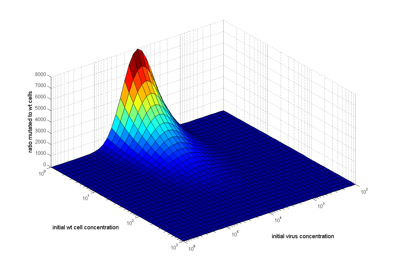
| - | For two dimensional analysis we changed two | + | For two dimensional analysis we changed two parameters, holding all other parameters constant at reference state and observed the ratio of mutated cells to wt cells. Two dimensional analysis can in this way show the influence of two parameters among each other. The analysis of initial virus concentration and wt cell concentration shows that there is an optimal virus concentration and the concentration of wt cells should be low (Figure 6). That the wt cell concentration should be very low make biologically no sense at all. The infection rates of virus show us that there is a wide range which leads to successful selection (Figure 7). But if infection rate for wt cell is too high and infection rate for mutated cell is too low we got no successful selection. |
| - | <table><tr><td>[[File:UP12_Modeling_detModel-initialC0andV0.png|left|300px|thumb|''' | + | <table><tr><td>[[File:UP12_Modeling_detModel-initialC0andV0.png|left|300px|thumb|'''Figure 6:''' Ratio mutated to wt cell concentration is plotted against initial wt cell and virus concentration.]] |
</td><td> | </td><td> | ||
| - | [[File:UP12_Modeling_detModel-kinfC-kinfM.png|left|300px|thumb|''' | + | [[File:UP12_Modeling_detModel-kinfC-kinfM.png|left|300px|thumb|'''Figure 7:''' Ratio mutated to wt cell concentration is plotted against infection rate for mutated and wt cell.]] |
</td></tr></table> | </td></tr></table> | ||
| - | ====== | + | ======Influence on time scale====== |
| - | To find out which parameter | + | To find out which parameter has an influence on time scale, we observed the ratio of mutated cells to wt cells over the time changing only one parameter. If the parameter has an influence on time scale, changes in the ratio of mutated cells to wt cells should be observed earlier or later. Following results were obtained: |
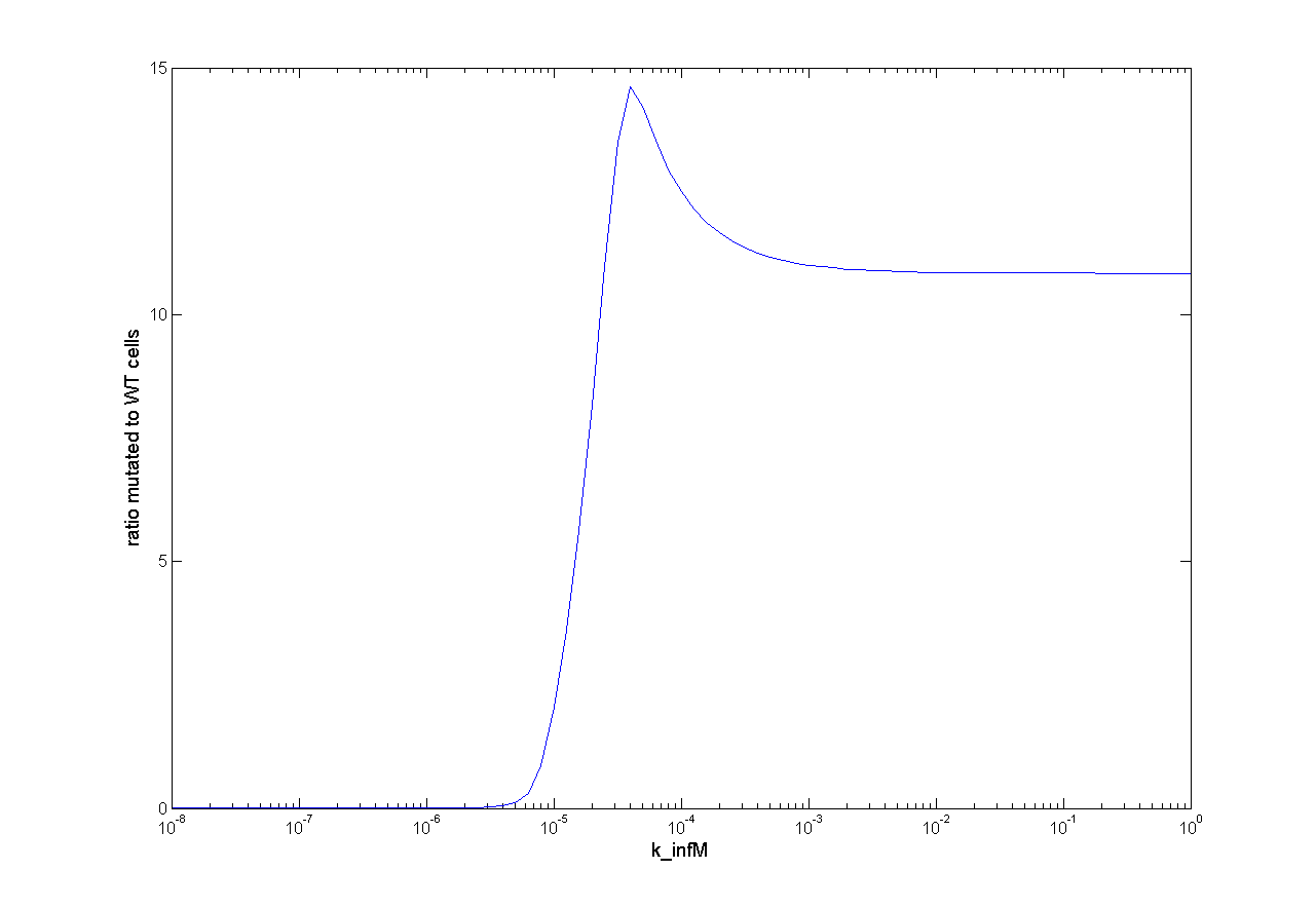
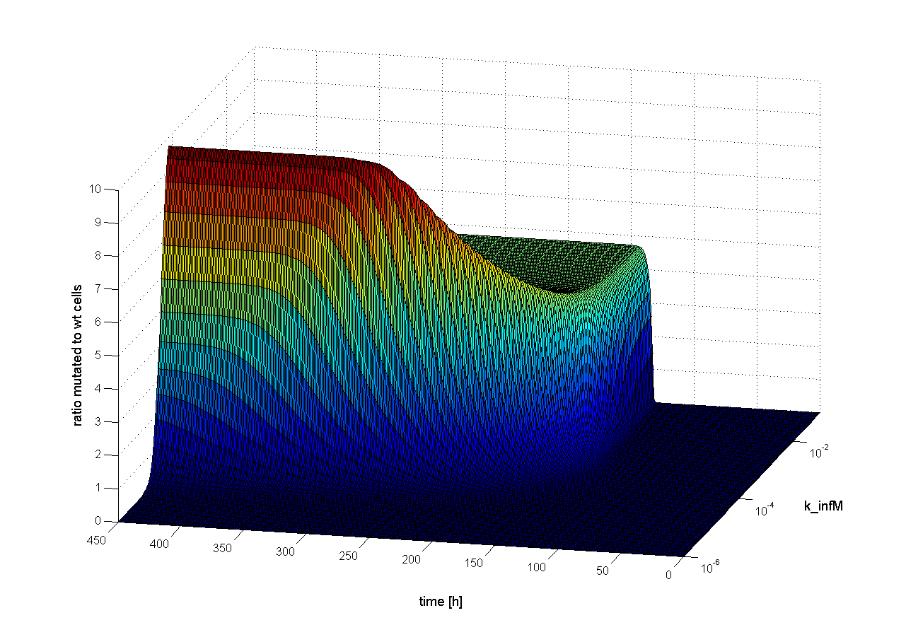
| - | We observed that different parameters have different influence on time flow of our selection systems. A high influence on time flow have the mutation rate (k_mut), the infection rate for mutated cells (k_infM) and the cell division rate after virus infection (k_divAinf). On Figure | + | We observed that different parameters have different influence on time flow of our selection systems. A high influence on time flow have the mutation rate (k_mut), the infection rate for mutated cells (k_infM) and the cell division rate after virus infection (k_divAinf). On Figure 8 for example you can see that the higher the mutation rate the earlier we get a higher ratio of mutated to WT cells. This means selection of mutated cells presenting a high affine antibody happens earlier. Also the higher the infection rate for mutated cells or the cell division after infection, the earlier we get a selection success (Figure 9 and 10). <br> |
<table> | <table> | ||
<tr><td> | <tr><td> | ||
| - | [[File:UP12_det-kmut.png|600px|left|thumb|'''Figure | + | [[File:UP12_det-kmut.png|600px|left|thumb|'''Figure 8:''' Influence on time scale of mutation rate. Ratio mutated to wt cell is plotted against parameter value and time.]] |
| - | [[File:UP12_det-kinfM.png|200px|left|thumb|'''Figure | + | [[File:UP12_det-kinfM.png|200px|left|thumb|'''Figure 9:''' Influence on time scale of infection rate of virus for mutated cell.]] |
| - | [[File:UP12_det-kdivAinf.png|200px|left|thumb|'''Figure | + | [[File:UP12_det-kdivAinf.png|200px|left|thumb|'''Figure 10:''' Influence on time scale of cell division rate after virus infection.]] |
</td></tr></table><table> | </td></tr></table><table> | ||
<tr><td> | <tr><td> | ||
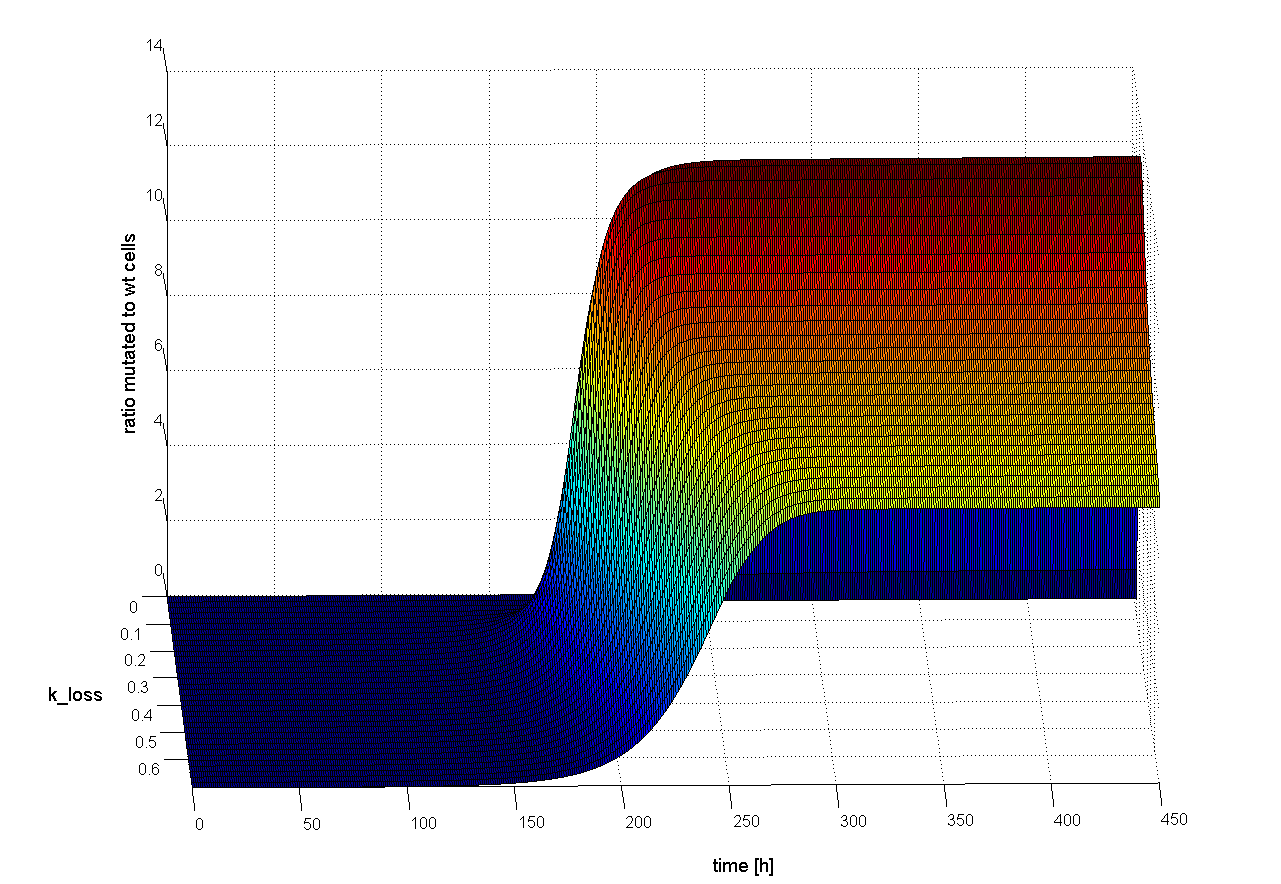
| - | The parameter k_loss have only low influence on time flow of selection system (see Figure | + | The parameter k_loss have only low influence on time flow of selection system (see Figure 11). The higher rate of the loss of viral genes (the positive signal), the later selection is successful. |
| - | The cell division rate (k_div), the cell death rate (k_death) and the infection rate with WT cells (k_infC) are time independent (see | + | The cell division rate (k_div), the cell death rate (k_death) and the infection rate with WT cells (k_infC) are time independent (see Figures 12-14). These parameters have only an influence on success of our selection system, but not on the time point when selection is finished. |
</td><td> | </td><td> | ||
| - | [[File:UP12_det-kloss.png|left|200px|thumb|'''Figure | + | [[File:UP12_det-kloss.png|left|200px|thumb|'''Figure 11:''' Influence on time scale of loss of viral genes]] |
</td><td> | </td><td> | ||
| - | [[File:UP12_det-kdiv.png|100px|left|thumb|'''Figure | + | [[File:UP12_det-kdiv.png|100px|left|thumb|'''Figure 12:''' Influence on time scale of cell division rate]] |
</td><td> | </td><td> | ||
| - | [[File:UP12_det-kdeath.png|100px|left|thumb|'''Figure | + | [[File:UP12_det-kdeath.png|100px|left|thumb|'''Figure 13:''' Influence on time scale of cell death rate]] |
</td><td> | </td><td> | ||
| - | [[File:UP12_det-kinfC.png|100px|left|thumb|'''Figure | + | [[File:UP12_det-kinfC.png|100px|left|thumb|'''Figure 14:''' Influence on time scale of infection rate of virus for wt cell.]] |
</td> | </td> | ||
</tr> | </tr> | ||
</table> | </table> | ||
| - | |||
| - | |||
| - | |||
| - | |||
| - | |||
| - | |||
====Stochastic Model==== | ====Stochastic Model==== | ||
| - | Stochastic modeling is necessary if one or more species occur in low amounts. In this case reactions are random events that lead to fluctuating concentrations of species which can be characterized by different results in several experiments or runs, respectively. In our selection system we get only low amount of mutated cells due to low mutation rate. Because of this and because of some peculiar behavior of the deterministic model we did stochastic modeling. For this we used the “simbiology” - tool of MATLAB. We built our model in the “simbiology” - tool and calculated stochastic kinetics using the stochastic simulation algorithm (SSA). This algorithm efficiently generates individual simulations that are consistent with the chemical master equation (CME). The greatest advantage of this algorithm is the precision. | + | Stochastic modeling is necessary if one or more species occur in low amounts. In this case reactions are random events that lead to fluctuating concentrations of species which can be characterized by different results in several experiments or runs, respectively. In our selection system we get only low amount of mutated cells due to low mutation rate. Because of this and because of some peculiar behavior of the deterministic model we did stochastic modeling. For this we used the “simbiology” - tool of MATLAB. We built our model in the “simbiology” - tool and calculated stochastic kinetics using the stochastic simulation algorithm (SSA). This algorithm efficiently generates individual simulations that are consistent with the chemical master equation (CME). The greatest advantage of this algorithm is the precision. |
We used the same parameters like in deterministic modeling. | We used the same parameters like in deterministic modeling. | ||
| Line 200: | Line 192: | ||
=====Results===== | =====Results===== | ||
| - | In figure | + | In figure 15 the concentration of each species is plotted against the time. We see nearly the same results compared to deterministic model. The concentrations of virus and WT cells decrease. From a certain time point the concentrations of infected mutated cells and mutated cells increase while virus is available. When virus concentration becomes zero, the concentrations of infected mutated cells and mutated cells decrease. |
| - | [[File:UP12_Modeling_stochModel-mainresult.png|center|700px|thumb|'''Figure | + | [[File:UP12_Modeling_stochModel-mainresult.png|center|700px|thumb|'''Figure 15:''' Solution of CME with stochastic simulation algorithm (SSA).]] |
| - | The difference between deterministic and stochastic model becomes obvious when we run the stochastic calculation several times (see figure | + | The difference between deterministic and stochastic model becomes obvious when we run the stochastic calculation several times (see figure 16). Figure 16 shows that the time point when mutated cells were selected and their concentration was greater than non-mutated cells, differ in large scales. Furthermore, in some runs mutated cells did not arise, meaning that sometimes the selection was not successful. This is a typical result and can be explained by the stochastic behavior. Because of low concentration of mutated cells sometimes they become extinct by random events and no selection takes place. |
| - | [[File:UP12_Modeling_stochModel-ensemblerun.png|center|700px|thumb|'''Figure | + | [[File:UP12_Modeling_stochModel-ensemblerun.png|center|700px|thumb|'''Figure 16:''' Example of ensemble run of our selection system. After 10 runs we got 7 successful selections]] |
=====Parameter Analysis===== | =====Parameter Analysis===== | ||
| - | For stochastic modeling we also | + | For stochastic modeling we also performed parameter analysis for both one and two dimensional. We change one or two parameters while holding the other parameters constant and run the calculation 3x100 times counting the successful selections. As a successful selection we defined a ratio of mutated cells to WT cells greater than 1. |
| - | In Figure | + | In Figure 17 you can see the results for 100 runs for different initial virus or wt cell concentration. For initial virus concentration you can see that at 100 virus particles per mL we got 0 successful selection. If we increase the concentration we got more positive results, but if the number of virus particles per mL was increased to 100000 particles/mL, the percentage of successful results decreases. Similar results were obtained for initial wt cell concentration.<br> |
[[Media:UP12-stoch-parameteranalysis.m]]<br> | [[Media:UP12-stoch-parameteranalysis.m]]<br> | ||
<html> | <html> | ||
| Line 246: | Line 238: | ||
</script> | </script> | ||
| + | |||
| Line 318: | Line 311: | ||
</td></tr></table> | </td></tr></table> | ||
</html> | </html> | ||
| - | |||
| - | |||
| + | '''Figure 17:''' 100 runs of stochastic model with different initial virus or wt cell concentration. Hover with cursor over the different concentrations to see results. | ||
| Line 327: | Line 319: | ||
With the ensemble runs we count the successful selection and plotted the percentage of successful selections against the parameter values for one dimensional analysis. | With the ensemble runs we count the successful selection and plotted the percentage of successful selections against the parameter values for one dimensional analysis. | ||
| + | <table border="1" rules="none"><tr><td> | ||
<table border="1" rules="none" align="center" cellspacing="0" cellpadding="0"> | <table border="1" rules="none" align="center" cellspacing="0" cellpadding="0"> | ||
| Line 345: | Line 338: | ||
</tr> | </tr> | ||
</table> | </table> | ||
| - | '''Figure | + | </td></tr><tr><td> |
| + | '''Figure 18:''' One dimensional analysis of all parameters. The percentage of selection success is plotted against the parameter value. | ||
| + | </td></tr></table> | ||
The one dimensional analysis shows nearly the same results like for deterministic model. The important difference is that initial wt cell concentration should not be to low. So there is an optimum wt concentration to get high probability for successful selection. This you also can see in two dimensional analysis together with initial virus concentration (see below). | The one dimensional analysis shows nearly the same results like for deterministic model. The important difference is that initial wt cell concentration should not be to low. So there is an optimum wt concentration to get high probability for successful selection. This you also can see in two dimensional analysis together with initial virus concentration (see below). | ||
| - | ====== | + | ======Two dimensional (2D)====== |
| - | There are optimal concentrations for virus and wt cells to get the highest probability for successful selection (see | + | There are optimal concentrations for virus and wt cells to get the highest probability for successful selection (see Figure 19). Both too high and too low concentration decrease the probability to get a positive result. But this optimum is influenced by several other parameters. For example if we increase the cell death rate we can increase the initial wt cell concentration (Figure 20). Through the high cell death rate, which is closed to high selection pressure, the mutated cells get a better chance to win recognition against wt cells. |
<table> | <table> | ||
<tr><td> | <tr><td> | ||
| - | [[File:UP12_Modeling_stochModel-initialC0andV0-01.png|left|500px|thumb|'''Figure | + | [[File:UP12_Modeling_stochModel-initialC0andV0-01.png|left|500px|thumb|'''Figure 19:'''Dependency of success form initial virus and wt cell concentrations.]] |
| - | [[File:UP12_Modeling_stochModel-initialC0andkdeath.png|left|300px|thumb|'''Figure | + | [[File:UP12_Modeling_stochModel-initialC0andkdeath.png|left|300px|thumb|'''Figure 20:'''Influence of cell death rate on optimal initial wt cell concentration.]] |
</td></tr></table> | </td></tr></table> | ||
| Line 362: | Line 357: | ||
With stochastic calculations we got the best results. The deterministic modeling had some strange behavoir, especially in parameter analysis. For example make the deterministic model the prediction that the initial wt cell concentration should be very low, but that is not biological realistic. Therefore stochastic modeling is much better. <br> | With stochastic calculations we got the best results. The deterministic modeling had some strange behavoir, especially in parameter analysis. For example make the deterministic model the prediction that the initial wt cell concentration should be very low, but that is not biological realistic. Therefore stochastic modeling is much better. <br> | ||
| - | Stochastic results showed that the selection is finished on random time points after 100 h or later ( | + | Stochastic results showed that the selection is finished on random time points after 100 h or later (Figure 16). The probability that selection is finished increases with time. |
| - | Furthermore, the analysis of initial concentrations of wt cell and virus revealed that there is an optimum for initial concentrations of wt cell and virus ( | + | Furthermore, the analysis of initial concentrations of wt cell and virus revealed that there is an optimum for initial concentrations of wt cell and virus (Figure 19). Both too less and too excessive concentrations prevent the success of the selection system. This optimum is influenced by the other parameters, but if we can determine some of these parameters we can calculate the optimal concentrations to start our selection. |
| + | |||
| + | ===MATLAB-Codes=== | ||
| + | |||
| + | [[Media:UP12-det-simplemodel.m]]<br> | ||
| + | [[Media:UP12-det-twostepmodel.m]]<br> | ||
| + | [[Media:UP12-det-parameteranalysis.m]]<br> | ||
| + | [[Media:UP12-stoch-parameteranalysis.m]]<br> | ||
| + | |||
</div> | </div> | ||
Latest revision as of 16:58, 26 October 2012
Contents |
Modeling
Introducion
Modeling is a powerful tool to understand complex interactions or processes. We created a model to illustrate our selection system and to get a better understanding of its behavior under different conditions. Thereby, we wanted to answer two main questions:
- At which time point selection is successful?
- How many antibody presenting cells and how many virus particles do we need at the beginning?
To answer these questions we did both deterministic and stochastic modeling using MATLAB. Furthermore, we did a huge parameter analysis for each model to check what kind of influence each parameter has on our selection system.
Simplest Model
Reaction Scheme
We built a simple model of our in vivo selection system which includes the reactions that are the most equivalent to our project. The following scheme (Figure 1) shows the reactions occurring in our model.
Species:
reaction rates:
|
Our system starts with the antibody presenting cell exhibiting a cell division rate (k_div) and a cell death rate (k_death). Due to expression of AID the antibodies get mutated and with a particular rate (k_mut) we get a mutated cell presenting more affine antibodies. Thereby, the virus infection is changed and is able to trigger the selection of mutated cells. We can distinguish between two different cases.
Within the first case, the infection rate of the virus to the mutated cell (kint_M) is improved compared to the infection rate to WT cell (kint_C). In this case through the virus infection a positive stimulus can be mediated, resulting in both a higher cell division rate (k_divAinf) and/or a lower cell death rate (k_deathAinf).
In case two, the infection rate of the virus to the mutated cell is decreased compared to the infection rate to WT cell C (k_intM < k_intC). Hence, through the virus infection, a negative stimulus can be mediated, resulting in a lower cell division rate (k_divAinf) or a higher cell death rate (kdeathAinf) or even both. The stimulus due to virus infection gets lost while the process proceeds (k_loss). This means that the virus infection is steadily required for those stimuli.
Due to the experimental observation which show that without an antibody no infection can be seen, we assume that with a better antibody on the cell surface the infection rate by the virus is improved compared to the WT cell. This means we should apply a positive selection system. For this we use antibiotics as selection pressure and antibiotic resistance as positive stimulus through virus infection. Therefore, for modeling we used low cell division rate compared to cell death rate and a high cell division rate after virus infection.
Deterministic Model
For deterministic modeling we write the reactions as ordinary differential equations (ODE´s) (Figure 2) and solved them using MATLAB. Because we only had marginal information about parameter values we estimate them and did a large parameter analysis (see below).
ODE´s
Results
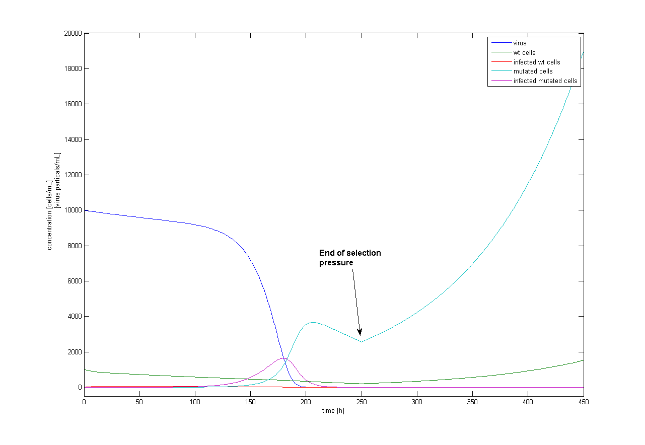
For calculation in MATLAB we used the following parameter values as reference state. In figure 3 time dependent concentrations of each species are shown.
Reference state:
|
We start with a 10-fold higher concentration of virus (shown in dark blue) compared to WT cell (shown in green). Concentration of WT cells decreases because of cell death due to antibiotic pressure. Virus concentration decreases because of infection of cells. WT cells were only marginal infected resulting in low concentration of infected WT cells (shown in red). After about 100 h mutated cells arose and were directly infected, because of high infection rate and high virus concentration. This leads to increased concentration of infected mutated cells and mutated cells respectively, due to stimulus of virus infection (antibiotic resistance). From that time point concentration of virus decreases rapidly and gets down to zero at about 200 h. Because of the lack of virus, cells were not infected and will get no positive stimulus. Due to continuous antibiotic pressure, cell concentration of both mutated and WT cells decreases.
To act against these decreases we performed two time steps (figure 4). In the first time step high selection pressure via antibiotics was applied. After successful selection, the antibiotic pressure was removed (e.g. by medium exchange) and therefore cell concentration increases due to higher cell division rate than cell death rate. Media:UP12-det-twostepmodel.m
Parameter Analysis
Because we had only marginal information about parameter values we did a large parameter analysis. We wanted to know how each parameter influences the selection system. Therefore, we looked at the influence on success of selection and the influence on time scale. For this analysis we observed the ratio of mutated cells to WT cells (ratio of M to C). For a successful selection the ratio of mutated cells to WT cells should be higher than one and as high as possible.
Media:UP12-det-parameteranalysis.m
One dimensional (1D)
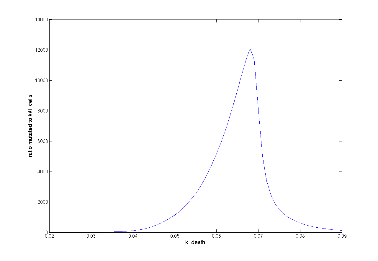
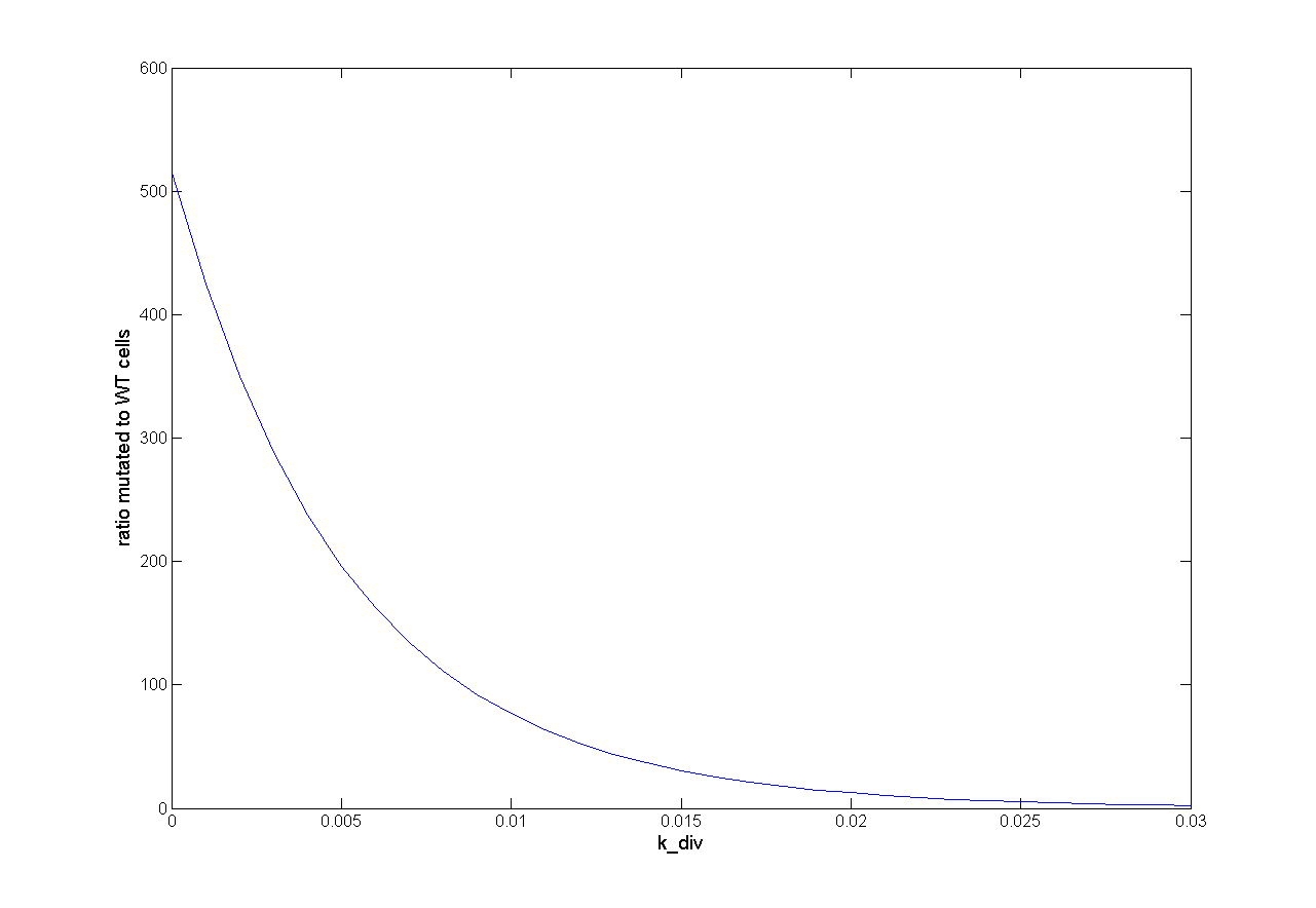
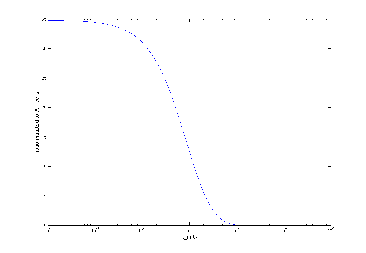
For one dimensional analysis we changed each parameter holding all other parameters constant at reference state and observed the ratio of mutated cells to WT cells. Following results were obtained:
|
| |||||||||
|
Figure 5: One dimensional analysis of all parameters. The ratio mutated to wt cells is plotted against the parameter value. A high ratio is related to successful selection. |
This parameter analysis gives us different information about the behavior of our selection system. Following highlights can be mentioned. For some of the parameters there exists an optimum range of parameter value for our model. One example is the initial virus concentration. Both too less and too excessive concentration prevent successful selection. Other parameters should be high or low. The mutation rate for example should be high to get a successful selection. The infection rate of the virus is also important. The infection rate for mutated cells must be higher than the infection rate for wt cells to get a positive result. A strange behavior is shown by the initial wt cell concentration. The model predicts that the lower the concentration, the better the selection. This is not biological reasonable and can be due to deterministic calculation. Therefore, we run stochastic calculation of our model (see below).
Two dimensional (2D)
For two dimensional analysis we changed two parameters, holding all other parameters constant at reference state and observed the ratio of mutated cells to wt cells. Two dimensional analysis can in this way show the influence of two parameters among each other. The analysis of initial virus concentration and wt cell concentration shows that there is an optimal virus concentration and the concentration of wt cells should be low (Figure 6). That the wt cell concentration should be very low make biologically no sense at all. The infection rates of virus show us that there is a wide range which leads to successful selection (Figure 7). But if infection rate for wt cell is too high and infection rate for mutated cell is too low we got no successful selection.
Influence on time scale
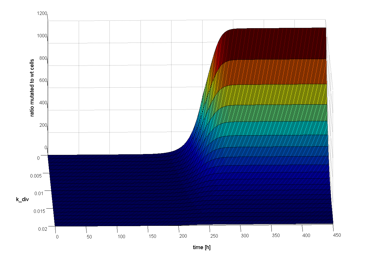
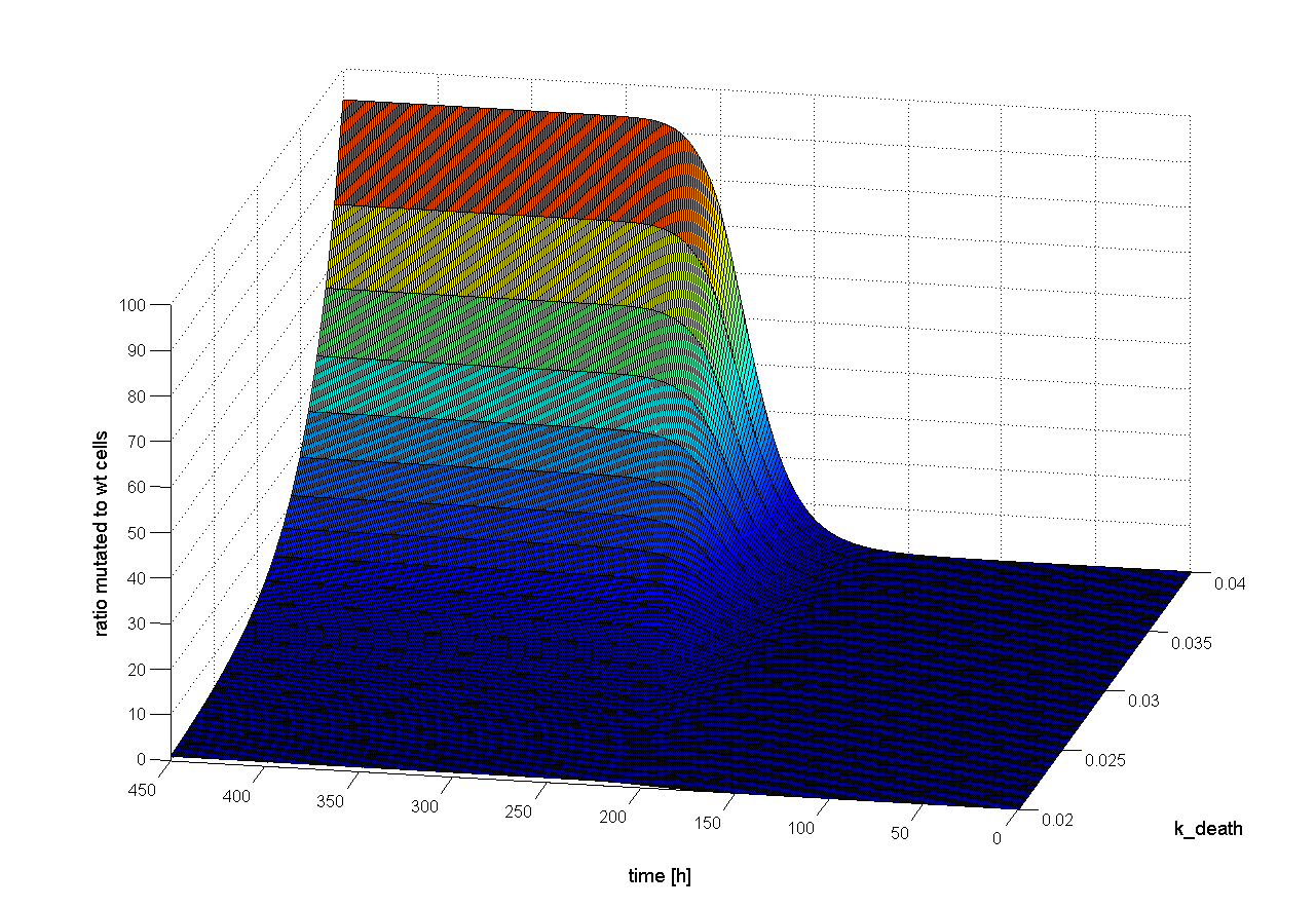
To find out which parameter has an influence on time scale, we observed the ratio of mutated cells to wt cells over the time changing only one parameter. If the parameter has an influence on time scale, changes in the ratio of mutated cells to wt cells should be observed earlier or later. Following results were obtained:
We observed that different parameters have different influence on time flow of our selection systems. A high influence on time flow have the mutation rate (k_mut), the infection rate for mutated cells (k_infM) and the cell division rate after virus infection (k_divAinf). On Figure 8 for example you can see that the higher the mutation rate the earlier we get a higher ratio of mutated to WT cells. This means selection of mutated cells presenting a high affine antibody happens earlier. Also the higher the infection rate for mutated cells or the cell division after infection, the earlier we get a selection success (Figure 9 and 10).
|
|
|
The parameter k_loss have only low influence on time flow of selection system (see Figure 11). The higher rate of the loss of viral genes (the positive signal), the later selection is successful. The cell division rate (k_div), the cell death rate (k_death) and the infection rate with WT cells (k_infC) are time independent (see Figures 12-14). These parameters have only an influence on success of our selection system, but not on the time point when selection is finished. |
Stochastic Model
Stochastic modeling is necessary if one or more species occur in low amounts. In this case reactions are random events that lead to fluctuating concentrations of species which can be characterized by different results in several experiments or runs, respectively. In our selection system we get only low amount of mutated cells due to low mutation rate. Because of this and because of some peculiar behavior of the deterministic model we did stochastic modeling. For this we used the “simbiology” - tool of MATLAB. We built our model in the “simbiology” - tool and calculated stochastic kinetics using the stochastic simulation algorithm (SSA). This algorithm efficiently generates individual simulations that are consistent with the chemical master equation (CME). The greatest advantage of this algorithm is the precision.
We used the same parameters like in deterministic modeling.
Results
In figure 15 the concentration of each species is plotted against the time. We see nearly the same results compared to deterministic model. The concentrations of virus and WT cells decrease. From a certain time point the concentrations of infected mutated cells and mutated cells increase while virus is available. When virus concentration becomes zero, the concentrations of infected mutated cells and mutated cells decrease.
The difference between deterministic and stochastic model becomes obvious when we run the stochastic calculation several times (see figure 16). Figure 16 shows that the time point when mutated cells were selected and their concentration was greater than non-mutated cells, differ in large scales. Furthermore, in some runs mutated cells did not arise, meaning that sometimes the selection was not successful. This is a typical result and can be explained by the stochastic behavior. Because of low concentration of mutated cells sometimes they become extinct by random events and no selection takes place.
Parameter Analysis
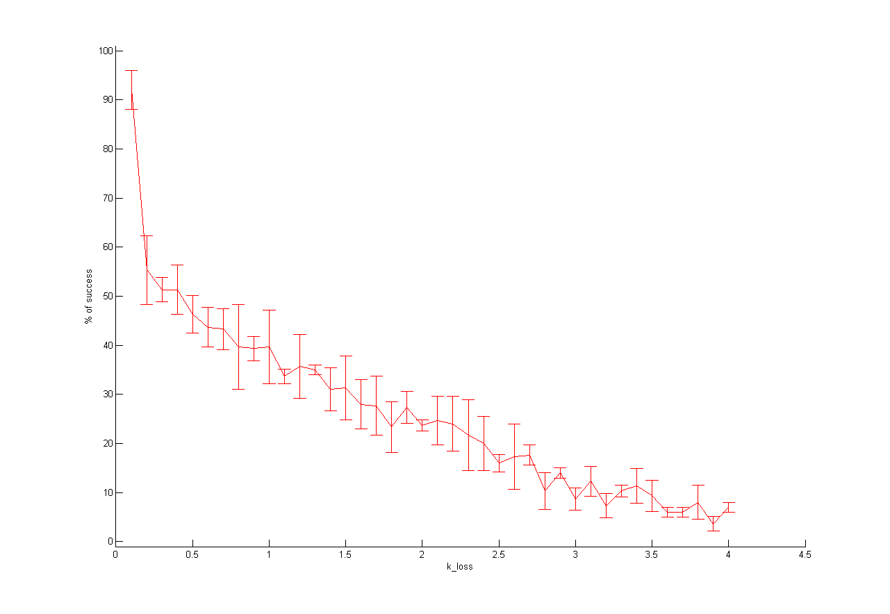
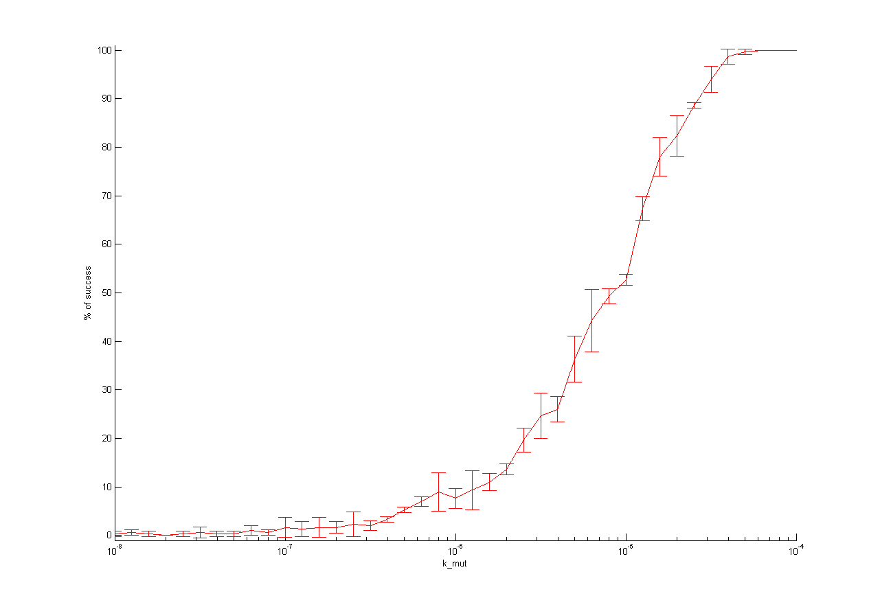
For stochastic modeling we also performed parameter analysis for both one and two dimensional. We change one or two parameters while holding the other parameters constant and run the calculation 3x100 times counting the successful selections. As a successful selection we defined a ratio of mutated cells to WT cells greater than 1.
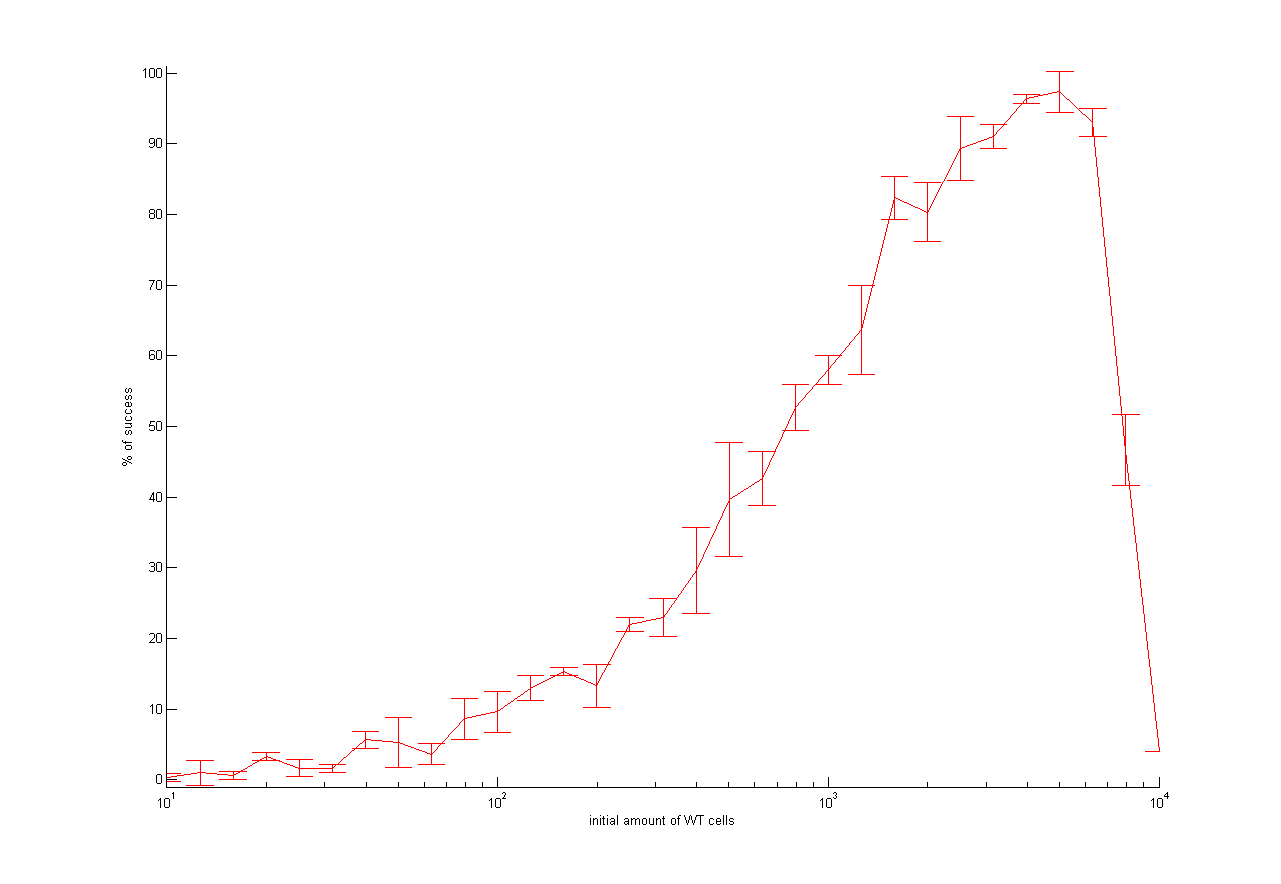
In Figure 17 you can see the results for 100 runs for different initial virus or wt cell concentration. For initial virus concentration you can see that at 100 virus particles per mL we got 0 successful selection. If we increase the concentration we got more positive results, but if the number of virus particles per mL was increased to 100000 particles/mL, the percentage of successful results decreases. Similar results were obtained for initial wt cell concentration.
Media:UP12-stoch-parameteranalysis.m

|

|
Figure 17: 100 runs of stochastic model with different initial virus or wt cell concentration. Hover with cursor over the different concentrations to see results.
One dimensional (1D)
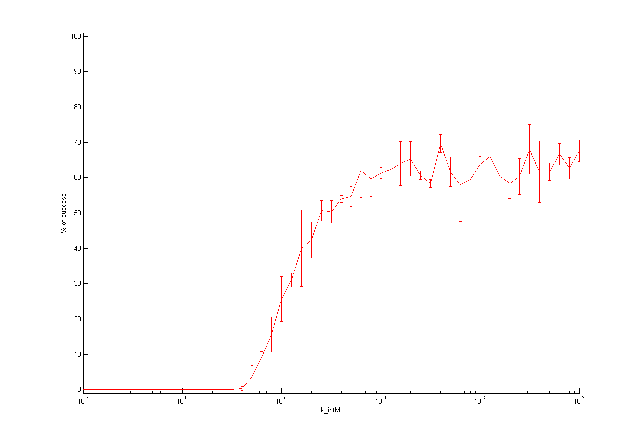
With the ensemble runs we count the successful selection and plotted the percentage of successful selections against the parameter values for one dimensional analysis.
|
| |||||||||
|
Figure 18: One dimensional analysis of all parameters. The percentage of selection success is plotted against the parameter value. |
The one dimensional analysis shows nearly the same results like for deterministic model. The important difference is that initial wt cell concentration should not be to low. So there is an optimum wt concentration to get high probability for successful selection. This you also can see in two dimensional analysis together with initial virus concentration (see below).
Two dimensional (2D)
There are optimal concentrations for virus and wt cells to get the highest probability for successful selection (see Figure 19). Both too high and too low concentration decrease the probability to get a positive result. But this optimum is influenced by several other parameters. For example if we increase the cell death rate we can increase the initial wt cell concentration (Figure 20). Through the high cell death rate, which is closed to high selection pressure, the mutated cells get a better chance to win recognition against wt cells.
Summary
With stochastic calculations we got the best results. The deterministic modeling had some strange behavoir, especially in parameter analysis. For example make the deterministic model the prediction that the initial wt cell concentration should be very low, but that is not biological realistic. Therefore stochastic modeling is much better.
Stochastic results showed that the selection is finished on random time points after 100 h or later (Figure 16). The probability that selection is finished increases with time.
Furthermore, the analysis of initial concentrations of wt cell and virus revealed that there is an optimum for initial concentrations of wt cell and virus (Figure 19). Both too less and too excessive concentrations prevent the success of the selection system. This optimum is influenced by the other parameters, but if we can determine some of these parameters we can calculate the optimal concentrations to start our selection.
MATLAB-Codes
Media:UP12-det-simplemodel.m
Media:UP12-det-twostepmodel.m
Media:UP12-det-parameteranalysis.m
Media:UP12-stoch-parameteranalysis.m
 "
"


