Team:USP-UNESP-Brazil/Associative Memory/Modeling
From 2012.igem.org
| (21 intermediate revisions not shown) | |||
| Line 13: | Line 13: | ||
</html> | </html> | ||
| - | <h1 id=" | + | <h1 id="model">Mathematical Model</h1> |
<p>We introduced a mathematical model for two populations of bacteria that interact via quorum sensing. Each population | <p>We introduced a mathematical model for two populations of bacteria that interact via quorum sensing. Each population | ||
produces its own quorum sensing molecule (QSM) and the QSM of one population can be repressive or excitatory to the other | produces its own quorum sensing molecule (QSM) and the QSM of one population can be repressive or excitatory to the other | ||
population in a mechanism analogous to a neuron communication. In our case, a neuron is represented by a population of | population in a mechanism analogous to a neuron communication. In our case, a neuron is represented by a population of | ||
| - | bacteria | + | bacteria whereas a synapse by a communication via QSM. In our analogy, a neuron is activated when the majority of the population |
| - | is in quorum, which means producing the QSM | + | is in quorum, which means producing the QSM at a high rate.</p> |
| - | |||
<p>Ward et al [1] introduced a mathematical model to describe the growth of populations of bacteria consisting in cell | <p>Ward et al [1] introduced a mathematical model to describe the growth of populations of bacteria consisting in cell | ||
| - | that can be either up-regulated or down-regulated. An up-regulated cell | + | that can be either up-regulated or down-regulated. An up-regulated cell produces QSM faster than a down-regulated cell, which |
| - | produces it in a basal rate. If the most bacteria in the population is up-regulated we say the population | + | produces it in a basal rate. If the most bacteria in the population is up-regulated, we say the population reached the quorum. |
| - | The model consists in | + | The model consists in the following differential equations:</p> |
\begin{align} | \begin{align} | ||
| Line 37: | Line 36: | ||
$A$ is the density of QSM, $\kappa_{d}$ and $\kappa_{u}$ are the QSM prodution rate of down-regulated and up-regulated, respectively. | $A$ is the density of QSM, $\kappa_{d}$ and $\kappa_{u}$ are the QSM prodution rate of down-regulated and up-regulated, respectively. | ||
The variable $\lambda$ is the degradation rate of the QSM and $r$ is the cell-division rate. | The variable $\lambda$ is the degradation rate of the QSM and $r$ is the cell-division rate. | ||
| - | It is assumed that down-regulated cells | + | It is assumed that down-regulated cells become up-regulated by QSMs with rate constant $\alpha$ and up-regulated becomes down-regulated |
with the rate $\beta$. | with the rate $\beta$. | ||
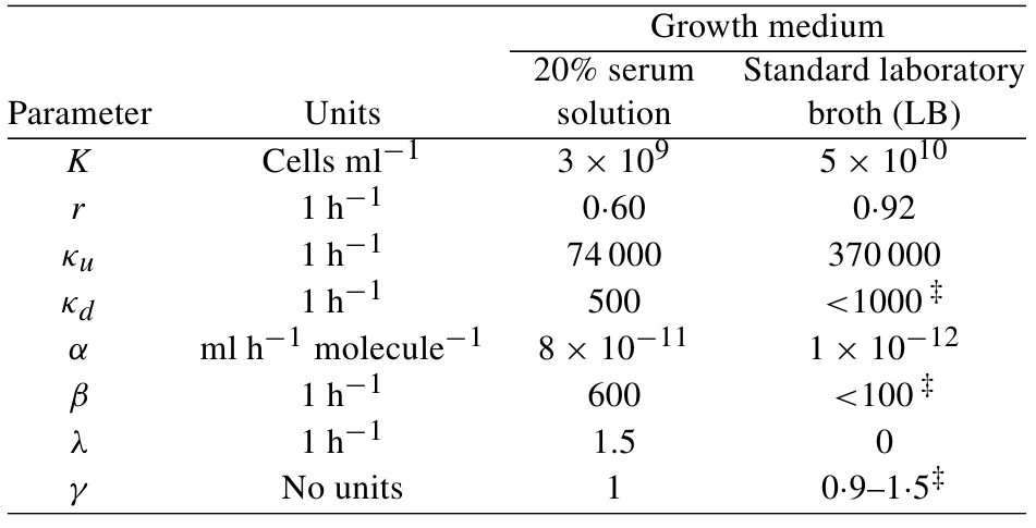
| - | + | {{:Team:USP-UNESP-Brazil/Templates/RImage | image=TableMatModelQS.jpeg | caption=Table. 1. Parameter values obtained by Ward et al [1]. | size=400px}} | |
| - | + | ||
| - | |||
| - | + | The authors designed some experiments in order to estimate the constants, Table 1. For example, the values for $K$ and $r$ were determined by examination of the growth curve. </p> | |
| - | + | ||
| - | Ward et al [1]. | + | |
| + | We proposed a model for two different types of population of bacteria by introducing an interaction between them in the model proposed by Ward et al [1]. | ||
| + | One population of bacteria are distinguishable of the other by the QSM that it produce. Lets call bacteria type A the population that produces QSM A and the same for B. | ||
| + | The interation is represented by an aditional term in the model that makes a type A up-regulated cells becomes down-regulated by QSM B with the rate | ||
$\phi_B$ and vice-versa. | $\phi_B$ and vice-versa. | ||
\begin{align} | \begin{align} | ||
| - | \frac{d}{dt}N_{Ad} &= rN_{At}\Big[1 - \frac{N_{At}}{K}\Big] - \alpha_A A N_{Ad} + | + | \frac{d}{dt}N_{Ad} &= rN_{At}\Big[1 - \frac{N_{At}}{K}\Big] - \alpha_A A N_{Ad} + \beta_A N_{Au} + \phi_B B N_{Au} \\ |
| - | \frac{d}{dt}N_{Bd} &= rN_{Bt}\Big[1 - \frac{N_{Bt}}{K}\Big] - \alpha_B A N_{Bd} + | + | \frac{d}{dt}N_{Bd} &= rN_{Bt}\Big[1 - \frac{N_{Bt}}{K}\Big] - \alpha_B A N_{Bd} + \beta_B N_{Bu} + \phi_A A N_{Bu} \\ |
\frac{d}{dt}N_{Au} &= \alpha_A A N_{Ad} - \beta_A N_{Au} - \phi_B B N_{Au}\\ | \frac{d}{dt}N_{Au} &= \alpha_A A N_{Ad} - \beta_A N_{Au} - \phi_B B N_{Au}\\ | ||
\frac{d}{dt}N_{Bu} &= \alpha_B B N_{Bd} - \beta_B N_{Bu} - \phi_A A N_{Bu} \\ | \frac{d}{dt}N_{Bu} &= \alpha_B B N_{Bd} - \beta_B N_{Bu} - \phi_A A N_{Bu} \\ | ||
| Line 62: | Line 62: | ||
<h1 id="model">Results</h1> | <h1 id="model">Results</h1> | ||
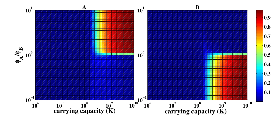
| - | We first evaluated the fraction of | + | We first evaluated the fraction of up-regulated cells as a function of the carrying capacity ($K$) and of the $\frac{\phi_A}{\phi_B}$ ratio, and $K$ turned out to be an important parameter of the model. For values of $K$ up to $10^8$, in the equilibrium, no population can reach the quorum state, since the density of cells is too low. On the other hand, for values higher than $10^8$ the population |
| + | that has a higher repression rate, represented by $\phi$, reaches quorum and represses the other population, as presented in Figure 1. | ||
| - | {{:Team:USP-UNESP-Brazil/Templates/RImage | image= | + | {{:Team:USP-UNESP-Brazil/Templates/RImage | image=KxRphis_alpha.jpg | caption=Fig. 1. The fraction of the up-regulated cells, for population A and B, as a function of the carrying capacity ($K$) and the ratio $\frac{\phi_A}{\phi_B}$ for the case $\phi_B = \alpha$, at equilibrium. Initial conditions: $N_{Au} = N_{Bu} = A = B = 0$. | size=620px}} |
| - | |||
| - | |||
| - | |||
| - | < | + | <h2 id="model">Equilibrium points </h2> |
| - | At | + | At equilibrium point, the equations 5 to 10 are equal to zero and thus: |
\begin{align} | \begin{align} | ||
| Line 86: | Line 84: | ||
\begin{align} | \begin{align} | ||
| - | + | \hspace{-0.5 cm} \frac{y(\kappa_{Bu} - \kappa_{Bd}) + \kappa_{Bd}}{\alpha_B (1-y) + \lambda^*_B + y\phi_B} = \frac{\Big[x(\kappa_{Au} - \kappa_{Ad}) + \kappa_{Ad}\Big]\alpha_A (1-x)} {\Big[\alpha_A (1-x) + \lambda^*_A + y\phi_A\Big]x\phi_B} - \frac{\beta_A}{\phi_B} \\ | |
| - | + | \hspace{-0.5 cm} \frac{x(\kappa_{Au} - \kappa_{Ad}) + \kappa_{Ad}}{\alpha_A (1-x) + \lambda^*_A + x\phi_A} = \frac{\Big[y(\kappa_{Bu} - \kappa_{Bd}) + \kappa_{Bd}\Big]\alpha_B (1-y)} {\Big[\alpha_B (1-y) + \lambda^*_B + x\phi_B\Big]y\phi_A} - \frac{\beta_B}{\phi_A} | |
\end{align} | \end{align} | ||
where $\lambda^* = \lambda/K$, and $x$ and $y$ range from 0 up to 1. These expressions are similar, since exchanging $A$ and $B$ turns one equation into the other. | where $\lambda^* = \lambda/K$, and $x$ and $y$ range from 0 up to 1. These expressions are similar, since exchanging $A$ and $B$ turns one equation into the other. | ||
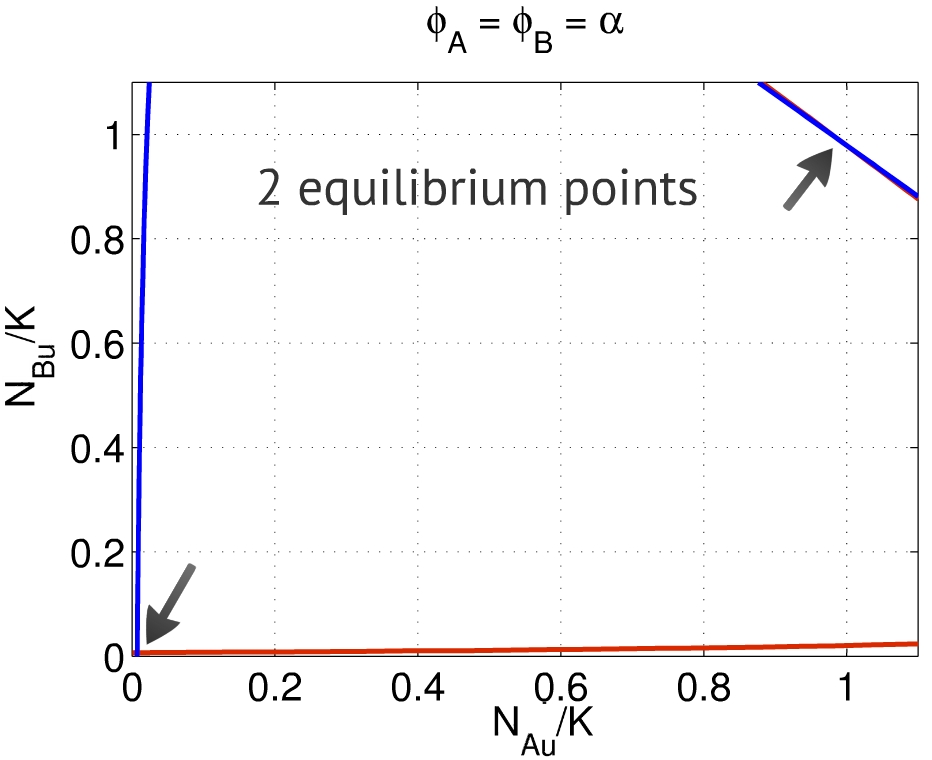
| - | + | {{:Team:USP-UNESP-Brazil/Templates/RImage | image=Phisiguais1.jpg | caption=Fig. 2. Each curve represents the solution of one equation, their intersections being the equilibrium points. One is close to $(0,0)$, the other to $(1,1)$. | size=350px}} | |
| - | + | Thus, the equilibrium points $(x,y)$ are placed in the intersection between the solutions for the relations above. Depending on the set of parameters, one can find two to four equilibria - the first one close to $(0,0)$, representing the repression of both populations, and the second one close to $(1,1)$, representing the activation of both populations, as presented in Fig. 2. In this case we used the parameters presented in Table 1, for 20% serum solution growth medium. The same behavior was found using the parameters for LB growth medium. | |
| + | We limitated the range of the variables $x$ and $y$ to [0,1] since it is the range that has a biological meaning. The entire curve can be seen in the following link [https://2012.igem.org/File:Phisiguais_2jpg.jpeg]. | ||
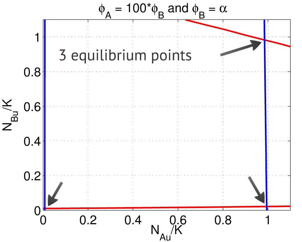
| - | + | {{:Team:USP-UNESP-Brazil/Templates/LImage | image=Phis100.jpg | left | caption=Fig. 3. When $\frac{\phi_A}{\phi_B} \gg 1$, besides the equilibria close to $(0,0)$ and $(1,1)$, there is also a point close to to $(1,0)$. | size=350px}} | |
| - | |||
| - | + | A third equilibrium point emerges when $\frac{\phi_A}{\phi_B} \gg 1$ - which means the repression of population A over population B is much greater than its counterpart, Fig. 3. In this case, the system also can reach an equilibrium close to $(1,0)$: population A activated, population B repressed. The behavior is analogous if $\frac{\phi_A}{\phi_B} \ll 1$. | |
| - | + | ||
| - | + | ||
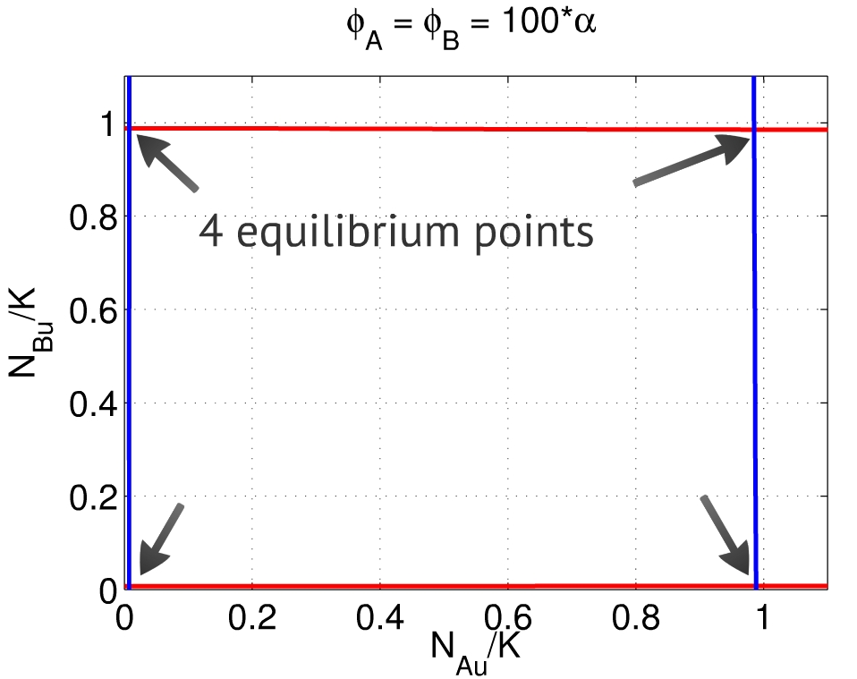
{{:Team:USP-UNESP-Brazil/Templates/RImage | image=Phis100ab.jpg | caption=Fig. 4. When $\frac{\phi_A}{\alpha_A} \gg 1$ and $\frac{\phi_B}{\alpha_B} \gg 1$, there are four equilibria, close to $(0,0)$, $(1,1)$, $(1,0)$ and $(0,1)$.} | size=350px}} | {{:Team:USP-UNESP-Brazil/Templates/RImage | image=Phis100ab.jpg | caption=Fig. 4. When $\frac{\phi_A}{\alpha_A} \gg 1$ and $\frac{\phi_B}{\alpha_B} \gg 1$, there are four equilibria, close to $(0,0)$, $(1,1)$, $(1,0)$ and $(0,1)$.} | size=350px}} | ||
| + | |||
| + | |||
| + | |||
| + | Finally, when both $\phi_A$ and $\phi_B$ are large when compared to $\alpha_A$ and $\alpha_B$, both populations A and B are able to | ||
| + | repress each other. In this case, the system can reach both equilibruim points $(1,0)$ and $(0,1)$ - repression | ||
| + | of one population and activation of the other, Fig. 4. This is the condition we should find experimentally in order to make our system works properly. | ||
| + | Its desired that, without any stimulus, the system converges to the point (0,0) and stays at this point. However, with a suficient stimulus the system should be able to converge to the point (0,1) or (1,0), depending on which population was stimulated. | ||
| + | |||
<h1 id="discussion">Discussion</h1> | <h1 id="discussion">Discussion</h1> | ||
| + | |||
| + | The Associative Memory Network project was based on a mathematical formulation of a neural network developed in 1982 by John Hopfield [3]. In order to connect the bacteria behavior during quorum sensing to a Hopfield network, we introduced an interaction between two populations in a mathematical model for quorum sensing. This interaction represents the neuronal repression/activation. Through steady-state analysis, it was possible to find up to four equilibrium points, representing the activation of both populations, activation of one population and repression of the other, and repression of both populations. The existence of these steady-state solutions depends on the set of parameters and stability analysis is being conducted to answer which regions in parameter space guarantee stability of each equilibria. | ||
| + | |||
| + | However, numerical simulations indicate that the carrying capacity $K$ is a fundamental parameter in the determination of the stability of quorum-state fixed points: changing its value had no effect on the location of these equilibria in $(x,y)$ space but, as shown in figure 1, increasing $K$ leads to quorum as a equilibrium point. Therefore, even though $K$ does not affect the existence of any fixed points, their stability seems to depend on its value - it would change a steady state from unstable to stable, so that for a population that would not reach quorum at a low carrying capacity might reach it when this parameter is increased. | ||
| + | |||
| + | In summary, the goal of this mathematical modeling has been achieved: it was verified that two bacterial populations are able to interact through repression and activation in order to reproduce a Hopfield Network. Additionally, different combinations of parameters and initial conditions may lead to different activation patterns: both populations activated, both repressed, or the asymetrical case - one up, one down. | ||
| + | |||
| + | Our further steps are to find the conditions for stability, which means to investigate the behaviour of the stable steady states as a function of the initial conditions - in other words, how the input changes the output. A network with more than two interacting populations is able to hold a systemic memory capable of storing and responding to a much wider range of patterns - a possibility that can be explored by our team in the future. | ||
| + | |||
<h1 id="references">References</h1> | <h1 id="references">References</h1> | ||
<p>[1] J. P. Ward, J.R. King, A. J. Koerber, P. Williams, J. M. Croft and R. E. Sockett | <p>[1] J. P. Ward, J.R. King, A. J. Koerber, P. Williams, J. M. Croft and R. E. Sockett | ||
| - | ''Mathematical modelling of quorum sensing in bacteria''. | + | ''Mathematical modelling of quorum sensing in bacteria''. |
| - | Math Med Biol (2001) 18(3) | + | Math Med Biol (2001) 18(3)</p> |
<p>[2] http://partsregistry.org/ </p> | <p>[2] http://partsregistry.org/ </p> | ||
| + | |||
| + | <p>[3] J. J. Hopfield. ''Neural networks and physical systems with emergent collective computational abilities''. Proceedings of the National Academy of Sciences of the USA, vol. 79 no. 8 pp. 2554–2558, April 1982.</p> | ||
{{:Team:USP-UNESP-Brazil/Templates/Foot}} | {{:Team:USP-UNESP-Brazil/Templates/Foot}} | ||
Latest revision as of 03:50, 27 September 2012
 Introduction
 Project Overview
 Plasmid Plug&Play
 Associative Memory
Network
 Extras
Contents |
Mathematical Model
We introduced a mathematical model for two populations of bacteria that interact via quorum sensing. Each population produces its own quorum sensing molecule (QSM) and the QSM of one population can be repressive or excitatory to the other population in a mechanism analogous to a neuron communication. In our case, a neuron is represented by a population of bacteria whereas a synapse by a communication via QSM. In our analogy, a neuron is activated when the majority of the population is in quorum, which means producing the QSM at a high rate.
Ward et al [1] introduced a mathematical model to describe the growth of populations of bacteria consisting in cell that can be either up-regulated or down-regulated. An up-regulated cell produces QSM faster than a down-regulated cell, which produces it in a basal rate. If the most bacteria in the population is up-regulated, we say the population reached the quorum. The model consists in the following differential equations:
\begin{align} \frac{d}{dt} N_{d} &= rN_{t}\Big[1 - \frac{N_{t}}{K}\Big] - \alpha A N_{d} + \beta N_{u} \\ \frac{d}{dt} N_{u} &= \alpha A N_{d} - \beta N_{u} \\ \frac{d}{dt} A &= \kappa_{u} N_{u} + \kappa_{d} N_{d} - \alpha A N_{d} - \lambda A \\ N_{t} &= N_{d} + N_{u} \end{align}
where $N_d$ and $N_u$ are the down-regulated and up-regulated subpopulations density (number of cells per volume), $A$ is the density of QSM, $\kappa_{d}$ and $\kappa_{u}$ are the QSM prodution rate of down-regulated and up-regulated, respectively. The variable $\lambda$ is the degradation rate of the QSM and $r$ is the cell-division rate. It is assumed that down-regulated cells become up-regulated by QSMs with rate constant $\alpha$ and up-regulated becomes down-regulated with the rate $\beta$.
We proposed a model for two different types of population of bacteria by introducing an interaction between them in the model proposed by Ward et al [1].
One population of bacteria are distinguishable of the other by the QSM that it produce. Lets call bacteria type A the population that produces QSM A and the same for B.
The interation is represented by an aditional term in the model that makes a type A up-regulated cells becomes down-regulated by QSM B with the rate
$\phi_B$ and vice-versa.
\begin{align} \frac{d}{dt}N_{Ad} &= rN_{At}\Big[1 - \frac{N_{At}}{K}\Big] - \alpha_A A N_{Ad} + \beta_A N_{Au} + \phi_B B N_{Au} \\ \frac{d}{dt}N_{Bd} &= rN_{Bt}\Big[1 - \frac{N_{Bt}}{K}\Big] - \alpha_B A N_{Bd} + \beta_B N_{Bu} + \phi_A A N_{Bu} \\ \frac{d}{dt}N_{Au} &= \alpha_A A N_{Ad} - \beta_A N_{Au} - \phi_B B N_{Au}\\ \frac{d}{dt}N_{Bu} &= \alpha_B B N_{Bd} - \beta_B N_{Bu} - \phi_A A N_{Bu} \\ \frac{d}{dt}A &= \kappa_{Au} N_{Au} + \kappa_{Ad} N_{Ad} - \alpha_A A N_{Ad} - \lambda_A A - \phi_A A N_{Bu} \\ \frac{d}{dt}B &= \kappa_{Bu} N_{Bu} + \kappa_{Bd} N_{Bd} - \alpha_B B N_{Bd} - \lambda_B B - \phi_B B N_{Au} \\ N_{At} &= N_{Ad}+N_{Au} \\ N_{Bt} &= N_{Bd}+N_{Bu} \end{align}
Results
We first evaluated the fraction of up-regulated cells as a function of the carrying capacity ($K$) and of the $\frac{\phi_A}{\phi_B}$ ratio, and $K$ turned out to be an important parameter of the model. For values of $K$ up to $10^8$, in the equilibrium, no population can reach the quorum state, since the density of cells is too low. On the other hand, for values higher than $10^8$ the population that has a higher repression rate, represented by $\phi$, reaches quorum and represses the other population, as presented in Figure 1.
Equilibrium points
At equilibrium point, the equations 5 to 10 are equal to zero and thus:
\begin{align} &-\alpha_A A N_{Ad} + \beta_A N_{Au} + \phi_B B N_{Au} &= 0 \\ &\kappa_{Au} N_{Au} + \kappa_{Ad} N_{Ad} - \alpha_A A N_{Ad} - \lambda_A A - \phi_A A N_{Bu} &= 0 \\ &-\alpha_B B N_{Bd} + \beta_B N_{Bu} + \phi_A A N_{Bu} &= 0 \\ &\kappa_{Bu} N_{Bu} + \kappa_{Bd} N_{Bd} - \alpha_B B N_{Bd} - \lambda_B B - \phi_B B N_{Au} &= 0 \\ &N_{Au} + N_{Ad} &= K \\ &N_{Bu} + N_{Bd} &= K \end{align}
These equations can be reduced to two expressions involving $x = N_{Au}/K$ and $y = N_{Bu}/K$:
\begin{align} \hspace{-0.5 cm} \frac{y(\kappa_{Bu} - \kappa_{Bd}) + \kappa_{Bd}}{\alpha_B (1-y) + \lambda^*_B + y\phi_B} = \frac{\Big[x(\kappa_{Au} - \kappa_{Ad}) + \kappa_{Ad}\Big]\alpha_A (1-x)} {\Big[\alpha_A (1-x) + \lambda^*_A + y\phi_A\Big]x\phi_B} - \frac{\beta_A}{\phi_B} \\ \hspace{-0.5 cm} \frac{x(\kappa_{Au} - \kappa_{Ad}) + \kappa_{Ad}}{\alpha_A (1-x) + \lambda^*_A + x\phi_A} = \frac{\Big[y(\kappa_{Bu} - \kappa_{Bd}) + \kappa_{Bd}\Big]\alpha_B (1-y)} {\Big[\alpha_B (1-y) + \lambda^*_B + x\phi_B\Big]y\phi_A} - \frac{\beta_B}{\phi_A} \end{align}
where $\lambda^* = \lambda/K$, and $x$ and $y$ range from 0 up to 1. These expressions are similar, since exchanging $A$ and $B$ turns one equation into the other.
Thus, the equilibrium points $(x,y)$ are placed in the intersection between the solutions for the relations above. Depending on the set of parameters, one can find two to four equilibria - the first one close to $(0,0)$, representing the repression of both populations, and the second one close to $(1,1)$, representing the activation of both populations, as presented in Fig. 2. In this case we used the parameters presented in Table 1, for 20% serum solution growth medium. The same behavior was found using the parameters for LB growth medium. We limitated the range of the variables $x$ and $y$ to [0,1] since it is the range that has a biological meaning. The entire curve can be seen in the following link [1].
A third equilibrium point emerges when $\frac{\phi_A}{\phi_B} \gg 1$ - which means the repression of population A over population B is much greater than its counterpart, Fig. 3. In this case, the system also can reach an equilibrium close to $(1,0)$: population A activated, population B repressed. The behavior is analogous if $\frac{\phi_A}{\phi_B} \ll 1$.
Finally, when both $\phi_A$ and $\phi_B$ are large when compared to $\alpha_A$ and $\alpha_B$, both populations A and B are able to repress each other. In this case, the system can reach both equilibruim points $(1,0)$ and $(0,1)$ - repression of one population and activation of the other, Fig. 4. This is the condition we should find experimentally in order to make our system works properly. Its desired that, without any stimulus, the system converges to the point (0,0) and stays at this point. However, with a suficient stimulus the system should be able to converge to the point (0,1) or (1,0), depending on which population was stimulated.
Discussion
The Associative Memory Network project was based on a mathematical formulation of a neural network developed in 1982 by John Hopfield [3]. In order to connect the bacteria behavior during quorum sensing to a Hopfield network, we introduced an interaction between two populations in a mathematical model for quorum sensing. This interaction represents the neuronal repression/activation. Through steady-state analysis, it was possible to find up to four equilibrium points, representing the activation of both populations, activation of one population and repression of the other, and repression of both populations. The existence of these steady-state solutions depends on the set of parameters and stability analysis is being conducted to answer which regions in parameter space guarantee stability of each equilibria.
However, numerical simulations indicate that the carrying capacity $K$ is a fundamental parameter in the determination of the stability of quorum-state fixed points: changing its value had no effect on the location of these equilibria in $(x,y)$ space but, as shown in figure 1, increasing $K$ leads to quorum as a equilibrium point. Therefore, even though $K$ does not affect the existence of any fixed points, their stability seems to depend on its value - it would change a steady state from unstable to stable, so that for a population that would not reach quorum at a low carrying capacity might reach it when this parameter is increased.
In summary, the goal of this mathematical modeling has been achieved: it was verified that two bacterial populations are able to interact through repression and activation in order to reproduce a Hopfield Network. Additionally, different combinations of parameters and initial conditions may lead to different activation patterns: both populations activated, both repressed, or the asymetrical case - one up, one down.
Our further steps are to find the conditions for stability, which means to investigate the behaviour of the stable steady states as a function of the initial conditions - in other words, how the input changes the output. A network with more than two interacting populations is able to hold a systemic memory capable of storing and responding to a much wider range of patterns - a possibility that can be explored by our team in the future.
References
[1] J. P. Ward, J.R. King, A. J. Koerber, P. Williams, J. M. Croft and R. E. Sockett Mathematical modelling of quorum sensing in bacteria. Math Med Biol (2001) 18(3)
[2] http://partsregistry.org/
[3] J. J. Hopfield. Neural networks and physical systems with emergent collective computational abilities. Proceedings of the National Academy of Sciences of the USA, vol. 79 no. 8 pp. 2554–2558, April 1982.
 "
"


