Team:Colombia/Modeling/Paramterers
From 2012.igem.org
Gutiloluis (Talk | contribs) |
|||
| (126 intermediate revisions not shown) | |||
| Line 3: | Line 3: | ||
{{https://2012.igem.org/User:Tabima}} | {{https://2012.igem.org/User:Tabima}} | ||
| + | <div class="right_box"> | ||
== Parameters of the equations == | == Parameters of the equations == | ||
| Line 9: | Line 10: | ||
There are three possible ways to find this parameters: | There are three possible ways to find this parameters: | ||
| + | |||
| + | <html> | ||
| + | <br> | ||
| + | </br> | ||
| + | </html> | ||
| + | |||
::i) Literature. There are a lot of studies trying to find biological parameters, such as basal rate of protein production, kinetic constants, Monod's constants, etc. Moreover, there are so many biological systems and only a few of them have been characterized. Thus, it is difficult to find the parameters that are needed. | ::i) Literature. There are a lot of studies trying to find biological parameters, such as basal rate of protein production, kinetic constants, Monod's constants, etc. Moreover, there are so many biological systems and only a few of them have been characterized. Thus, it is difficult to find the parameters that are needed. | ||
| + | |||
| + | <html> | ||
| + | <br> | ||
| + | </br> | ||
| + | </html> | ||
| + | |||
::ii) Experimental way. If an experiment is made using the biological system of interest, it is possible to find the parameters for the equations that models the whole system. For this project, it was necessary to model the biological system first. Thus, experiments couldn't be performed to find the constant for the differential equations. | ::ii) Experimental way. If an experiment is made using the biological system of interest, it is possible to find the parameters for the equations that models the whole system. For this project, it was necessary to model the biological system first. Thus, experiments couldn't be performed to find the constant for the differential equations. | ||
| - | |||
| + | <html> | ||
| + | <br> | ||
| + | </br> | ||
| + | </html> | ||
| + | |||
| + | |||
| + | ::iii) Screening of parameters. Sometimes we don't have the exact number that we need, but we have a rank where it could be or the parameter for a similar biological system, then we can perfom a screening of parameter, where we try to find the value that perfectly fits the reponse of our circuit. | ||
== How did we do it? == | == How did we do it? == | ||
| - | |||
| - | We used a lot of resources and methods to approximate the limits for this ranges | + | <p align="justify"> |
| + | |||
| + | '''As said above finding the right set of parameters for a system is a headache for all the synthetic biologists. That is why we developed a standard procedure that can be use any synthetic biology mathematical model. It has four main steps. But before starting to work in it we need to find as much information in literature as possible.''' | ||
| + | |||
| + | |||
| + | <br> | ||
| + | <br> | ||
| + | |||
| + | For our particular case, ee found all the CI promoter box parameters, we normalized all the degradation terms with the cell division time and for the other we found acceptable ranges. We used a lot of resources and methods to approximate the limits for this ranges. Here we show an explanation: | ||
[[File:tabla2.png|center|300x250pxpx]] | [[File:tabla2.png|center|300x250pxpx]] | ||
| Line 24: | Line 50: | ||
'''''a.Basal levels of the proteins:''''' | '''''a.Basal levels of the proteins:''''' | ||
| - | + | Determining a rank which this value could be, we described mathematically a very simple process. Suppose there is a usual differential equation: | |
| - | [[File: | + | [[File:alfbsal1.png|center|120x120px]] |
| - | Where αo is the basal level, γ is the protein parameter for degradation and P is the protein concentration | + | Where αo is the basal level, γ is the protein parameter for degradation and P is the protein concentration. Thus, we can assume that in steady state conditions we have that dP/dt= 0: |
[[File:alfbasal2.png|center|80x60pxpx]] | [[File:alfbasal2.png|center|80x60pxpx]] | ||
| - | But γ is approximately 1/T, | + | But γ is approximately 1/T, then: |
[[File:alfbasal3.png|center|80x60pxpx]] | [[File:alfbasal3.png|center|80x60pxpx]] | ||
| - | + | Establishing the rank, we assumed T as φ and we looked for a normal rank of concentration of a protein in a cell [http://bionumbers.hms.harvard.edu/bionumber.aspx?&id=104520&ver=10&trm=protein]. Another important aspect is that there were constitutive proteins and inducible proteins. Thus, we divided the basal levels in two class: i) one for basal proteins and ii) one for constitutive proteins. Finally, following ranges were defined: | |
Basal proteins range (LuxR, LuxI, HipB and Salicylic Acid): | Basal proteins range (LuxR, LuxI, HipB and Salicylic Acid): | ||
| - | [[File:range1.png|center| | + | [[File:range1.png|center|156x104pxpx]] |
| - | + | ||
| - | + | ||
| - | + | Constitutive proteins range (HipA7,Sensor, Chitinase, Chitoporin and CBP): | |
| - | By other | + | [[File:z.png|center|153x105pxpx]] |
| + | |||
| + | By the other hand, the basal production of HipA has to be constitutive and inducible because the cell has to have three stages. The first stage is always sleep (constitutive) due to HipA effect. Once an impulse of chitin or 3-OH-PAME is presented, it is going to awake the cell due to concentration decrease of HipA . This is the second stage of the cell. The third stage is when cell is slept again which it is achieve through a positive control (inducible). The basal concentration used in the equations was the constitutive one because it is going to have more effect in the response. | ||
'''b.Protein degradation:''' | '''b.Protein degradation:''' | ||
| - | + | The chosen unit of time was the bacteria life time because it represents when the proteins are diluted and decrease in the cell. We can establish easily the protein degradation using values related to life time of E.Coli. We defined the protein degradation for almost all values as follows: | |
[[File:degrada.png|center|100x80pxpx]] | [[File:degrada.png|center|100x80pxpx]] | ||
| - | Again we | + | Again, we found a special case. Degradation of HB is greater, then we assigned it a value of 4/φ. |
'''c. Reaction constant:''' | '''c. Reaction constant:''' | ||
| - | This value can vary | + | This value can vary depending of the described process. Fortunately, we found in literature how to approximate this value [http://www.biokin.com/dynafit/scripting/html/node23.html#SECTION00431000000000000000]. However, we took the approximation and turned it into units described above. |
| + | |||
| + | [[File:reactioncte.png|center|186x126pxpx]] | ||
| + | |||
| + | '''d. Hill coefficients k:''' | ||
| + | |||
| + | We looked for some reference in different data sources and we found the coefficient of CI ([http://www.sciencemag.org/content/307/5717/1962.short Nitzal et al.2005]). Then, we decided to approximate a rank taking this value as a reference. | ||
| + | |||
| + | [[File:zzzzzzz.png|center|145x95pxpx]] | ||
| + | |||
| + | '''e. Hill coefficients n:''' | ||
| + | |||
| + | We based on the value "n" found for CI( [http://www.sciencemag.org/content/307/5717/1962.short NItzal et al.2005]). In this case, there was an analysis that took in account the number of molecules that interfere with gene activation. | ||
| + | |||
| + | [[File:zzzzRRzzz.png|center|260x172pxpx]] | ||
| + | |||
| + | '''f. Maximum cell production (β):''' | ||
| + | |||
| + | Considering the concentration of Rubisco, which is about 20 times the average concentration and rate of production of a protein, [http://bionumbers.hms.harvard.edu/bionumber.aspx?&id=107431&ver=1&trm=rubisco], we assign the limits for this range as follows. | ||
| + | |||
| + | [[File:RRMoizzz.png|center|136x90pxpx]] | ||
| + | |||
| + | '''CI PARAMETERS''' | ||
| + | |||
| + | All the parameters for CI activation system were found in the literature. ([http://www.sciencemag.org/content/307/5717/1962.short Nitzal et al.2005]). We only made a change of units. | ||
| + | |||
| + | [[File:CI.png|center|150x150pxpx]] | ||
| + | |||
| + | |||
| + | ---- | ||
| + | |||
| + | Once the ranges of the parameters were set, we proceed to develop the standard method. Here we show the steps proposed with the obtained results for Pest-busters as an example. | ||
| + | |||
| + | |||
| + | :'''Step 1: Objective function: Define your desired behavior''' | ||
| + | |||
| + | First of all, it is necesary to define the desired response, in this case the Salicylic Acid. Thus, we stablished some ranges where concentration supposed to be. This response depends on the chitin or 3-OH-PAME impulse. Besides, the system is preferable to respond if the signal is long and intense. On the other hand, we don't want our cells to be "awake". The figure below shows this: | ||
| + | |||
| + | [[File:param4.png|center|thumb|480x450pxpx|Figure 1. Objective function and desired behavior]] | ||
| + | |||
| + | |||
| + | :'''Step 2. Optimization of parameters: A point within an area''' | ||
| + | |||
| + | Within the parameter space, there are many sets of them that make the system behaves just like expected; and these can be represented as an area. The main objective is to find this area. Suppose you only have two parameters. The plane represents the parameter space and the green area is where the system works. | ||
| + | |||
| + | [[File:param.png|center|thumb|400x200pxpx|Figure 2. Parameter space for a system ]] | ||
| + | |||
| + | Now we want a point within these area to begin the screening. It seems easy to identify in two dimensions, but this process can take a lot of time (weeks or even months) when it is a space of more than 10 parameters. So, one way to achieve this process is making an optimization. | ||
| + | |||
| + | [[File:param2.png|center|thumb|400x200pxpx|Figure 3. A point in parameter space for a system]] | ||
| + | |||
| + | A process of optimization takes a function and found maximum or minimum values changing some variables of it. The changing variables are named optimization variables and function is called objective function. If we have some limitations, it is possible to add restrictions to the system, and the function will be optimized without breaking them. | ||
| + | |||
| + | In this case, the objective function is a minimum difference of squares between the points of the expected behavior and the response of the equations with a set of optimization variables. When the distance between these points is minimum, the parameters are found. | ||
| + | |||
| + | This optimization process was done discretizing the differential equations and putting them as restrictions. The same procedure was made for the stable state concentration where the differential equation must be equal to zero (when there is no signal). This algorithm was programmed in a specialized software. | ||
| + | |||
| + | Unfortunately the firsts results were not satisfactory and a new code it is being developed. | ||
| + | |||
| + | <br> | ||
| + | |||
| + | :'''Step 3: Sensitivity anlysis''' | ||
| + | |||
| + | In this step the importance of each parameters in the main outputs behavior (Our case: Salicylic Acid, the toxin HipA7 and the antitoxin HipB) is tested. The objective is to find how much each parameter affect the desired response. | ||
| + | |||
| + | This test considered the following stages: i.) Establish the ranges of the parameters (see above), ii) Determine appropriate division for the ranges, iii) Iterate each parameter while leaving the others fixed in the MATLAB code. iv) See how the difference between the steady state's concentrations and the concentrations during the impulse of the pathogen changed with the change of each parameter. | ||
| + | |||
| + | <br> | ||
| + | |||
| + | '''Note: the exact value for each parameter is not important. It is important their relevance and how they change the response.''' | ||
| + | |||
| + | <br> | ||
| + | |||
| + | Here is an example: | ||
| + | |||
| + | [[File:luxi.png|center|thumb|350x350pxpx|Figure 4. LuxI, maximal production rate. Range: 0-22. Step size: 0.5 ]] | ||
| + | |||
| + | <br> | ||
| + | |||
| + | The figure above shows how the HipB, HipA7 and Salicylic Acid concentration change during the presence of the pathogen is significantly influenced by the maximal production rate of LuxI protein. We make this procedure for all the parameters in both systems (Ralstonia and Fungus). The results are shown below: | ||
| + | |||
| + | <br> | ||
| + | |||
| + | ---- | ||
| + | |||
| + | '''Fungus:''' | ||
| + | |||
| + | The sensitivity analysis was performed for the system with the fungal detection module. The following table shows the different parameters involved in the system with the fungal detection module. Besides, it shows how they affect the final behavior. | ||
| + | |||
| + | [[File:resultsab.png|center|thumb|480x650pxpx|Table 1. Parameters involved in the fungal detection module]] | ||
| + | |||
| + | Here we present some of the graphics found in the analysis. The figures below show two parameters that do not have significant influence in the desired response: | ||
| + | |||
| + | [[File:funnochange.png|center|thumb|650x380pxpx|Figure 5. Parameters that do not have influence in the response]] | ||
| + | |||
| + | <br> | ||
| + | |||
| + | We also found some parameters that have a significant influence in one of the main outputs but were not sensitive to the rest: | ||
| + | |||
| + | [[File:funnochangeone.png|center|thumb|650x380pxpx|Figure 6. Parameters that have influence in the response ]] | ||
| + | |||
| + | Finally, we found some parameters that affect the final response of all the main outputs of interest: | ||
| + | |||
| + | [[File:funnochangetwo.png|center|thumb|650x380pxpx|Figure 7. Parameters that affect the final response]] | ||
| + | |||
| + | |||
| + | '''Ralstonia''' | ||
| + | |||
| + | Below, it is exposed the results obtained from sensitivity test for Ralstonia. The next table identifies those parameters that make a relevant change in the model from those that do not. The main outputs tested were the HipB, HipA7 and the salicylic acid change in concentration due to the impulse. | ||
| + | |||
| + | [[File:resultsabn3.png|center|thumb|480x650pxpx|Table 2. Parameters involved in Ralstonia detection module]] | ||
| + | |||
| + | The following figures show the results obtained for almost all the relevant parameters. Like in the previous case we found some parameters that had no effect at all in the response and others than only had effect in one of the main outputs. | ||
| + | |||
| + | [[File:ralchangeone.png|center|thumb|650x380pxpx|Figure 8. Behavior of relevant parameters for Ralstonia detection module]] | ||
| + | |||
| + | We also found some interesting results, there were some parameters that had a significant influence in a small range, but when the rest of the range was evaluated the response was not sensitive to these parameters: | ||
| + | |||
| + | [[File:ralchangetwo.png|center|thumb|650x380pxpx|Figure 9. Parameters that had a significant influence ]] | ||
| - | + | Finally we found parameters that had significant influence in the response of the three main outputs and in the complete range of the parameter. Here we present some of the most interesting behaviors of these kind of parameters: | |
| + | [[File:ralchange3.png|center|thumb|650x380pxpx|Figure 10. Parameters with significant influence]] | ||
| - | |||
| - | + | Using this results it is possible to know the parameters that affect the response in a major way. Although it is still unknown the exact value of the parameter, it is possible predict how the system is supposed to response. Then, we could proceed to the final step. | |
| + | <br> | ||
| + | :'''Step 4: Screening''' | ||
| - | + | ::''If we have a set of parameters, why do we do a screening?'' | |
| - | + | In the second step we found a set of parameters that give the expected response of the system. But this is only a point. What does happen with the rest of points of the area? Does the optimization method “know” if these parameters are real or have biological sense? As long as we specified one single response for the parameters, we don’t know if there are other possible responses of valid solutions. Do they exist? | |
| + | To answer these questions we performed a screening of the parameters. Beginning at the resulting point of the optimization, we started to move in all directions in a fixed range and then we examined when the acceptable area ends. | ||
| + | How much do we move depends on the sensitivity analysis. If the response is not very sensitive to the parameter, we take longer steps than the case which the response is more sensitive. | ||
| - | + | [[File:param3.png|center|thumb|400x200pxpx|Figure 11. Size of the steep for screening ]] | |
| - | + | There are some parameters that can me modified experimentally like the maximal rate production but most of them depend on molecular details, are unchangeable and can only be known with experiments. The final goal of these standard procedure is to set the changeable parameters in such a way that the cross sectional area of the area of parameters that has desired response is maximized. | |
| - | + | Suppose you only have two parameters, one that can be changed and one that does not. If you set the first parameter in a black dot (see figure below), a small change of the uncontrollable parameter would take the system out of its working area. The optimum solution is to set the first parameter in the red line, so the probability of going out of the working area is smaller. | |
| - | + | [[File:param5.png|center|thumb|500x300pxpx|Figure 12. Optimum solution for a system]] | |
| + | In the first trial we got this results | ||
| - | : | + | [[File:Seed.png|center|thumb|700x350pxpx|Figure 13. Volume with the desired response within the parameter space]] |
| - | : | + | [[File:Seed2.png|center|thumb|700x350pxpx|Figure 14. Volume with the desired response within the parameter space]] |
| - | + | ''We made a screening with very few steps because of the little computational time, which results are shown on section 4. At this moment we are running a screening with more steps in order to make it more precise.'' | |
| + | </p> | ||
| - | + | </div> | |
Latest revision as of 04:01, 27 October 2012
Team Colombia @ 2012 iGEM
Template:Https://2012.igem.org/User:Tabima
Parameters of the equations
When we want to model a biological process, it is necessary to write the differential equation that model the system which requires a number of constants. If the real value for the constants are unknown, the system can not have any biological sense. These entries are called parameters and they are crucial elements in the mathematical model made in this project.
There are three possible ways to find this parameters:
- i) Literature. There are a lot of studies trying to find biological parameters, such as basal rate of protein production, kinetic constants, Monod's constants, etc. Moreover, there are so many biological systems and only a few of them have been characterized. Thus, it is difficult to find the parameters that are needed.
- ii) Experimental way. If an experiment is made using the biological system of interest, it is possible to find the parameters for the equations that models the whole system. For this project, it was necessary to model the biological system first. Thus, experiments couldn't be performed to find the constant for the differential equations.
- iii) Screening of parameters. Sometimes we don't have the exact number that we need, but we have a rank where it could be or the parameter for a similar biological system, then we can perfom a screening of parameter, where we try to find the value that perfectly fits the reponse of our circuit.
How did we do it?
As said above finding the right set of parameters for a system is a headache for all the synthetic biologists. That is why we developed a standard procedure that can be use any synthetic biology mathematical model. It has four main steps. But before starting to work in it we need to find as much information in literature as possible.
For our particular case, ee found all the CI promoter box parameters, we normalized all the degradation terms with the cell division time and for the other we found acceptable ranges. We used a lot of resources and methods to approximate the limits for this ranges. Here we show an explanation:
a.Basal levels of the proteins:
Determining a rank which this value could be, we described mathematically a very simple process. Suppose there is a usual differential equation:
Where αo is the basal level, γ is the protein parameter for degradation and P is the protein concentration. Thus, we can assume that in steady state conditions we have that dP/dt= 0:
But γ is approximately 1/T, then:
Establishing the rank, we assumed T as φ and we looked for a normal rank of concentration of a protein in a cell [http://bionumbers.hms.harvard.edu/bionumber.aspx?&id=104520&ver=10&trm=protein]. Another important aspect is that there were constitutive proteins and inducible proteins. Thus, we divided the basal levels in two class: i) one for basal proteins and ii) one for constitutive proteins. Finally, following ranges were defined:
Basal proteins range (LuxR, LuxI, HipB and Salicylic Acid):
Constitutive proteins range (HipA7,Sensor, Chitinase, Chitoporin and CBP):
By the other hand, the basal production of HipA has to be constitutive and inducible because the cell has to have three stages. The first stage is always sleep (constitutive) due to HipA effect. Once an impulse of chitin or 3-OH-PAME is presented, it is going to awake the cell due to concentration decrease of HipA . This is the second stage of the cell. The third stage is when cell is slept again which it is achieve through a positive control (inducible). The basal concentration used in the equations was the constitutive one because it is going to have more effect in the response.
b.Protein degradation:
The chosen unit of time was the bacteria life time because it represents when the proteins are diluted and decrease in the cell. We can establish easily the protein degradation using values related to life time of E.Coli. We defined the protein degradation for almost all values as follows:
Again, we found a special case. Degradation of HB is greater, then we assigned it a value of 4/φ.
c. Reaction constant:
This value can vary depending of the described process. Fortunately, we found in literature how to approximate this value [http://www.biokin.com/dynafit/scripting/html/node23.html#SECTION00431000000000000000]. However, we took the approximation and turned it into units described above.
d. Hill coefficients k:
We looked for some reference in different data sources and we found the coefficient of CI ([http://www.sciencemag.org/content/307/5717/1962.short Nitzal et al.2005]). Then, we decided to approximate a rank taking this value as a reference.
e. Hill coefficients n:
We based on the value "n" found for CI( [http://www.sciencemag.org/content/307/5717/1962.short NItzal et al.2005]). In this case, there was an analysis that took in account the number of molecules that interfere with gene activation.
f. Maximum cell production (β):
Considering the concentration of Rubisco, which is about 20 times the average concentration and rate of production of a protein, [http://bionumbers.hms.harvard.edu/bionumber.aspx?&id=107431&ver=1&trm=rubisco], we assign the limits for this range as follows.
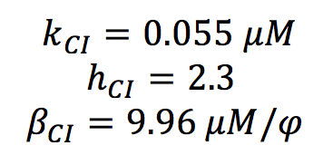
CI PARAMETERS
All the parameters for CI activation system were found in the literature. ([http://www.sciencemag.org/content/307/5717/1962.short Nitzal et al.2005]). We only made a change of units.
Once the ranges of the parameters were set, we proceed to develop the standard method. Here we show the steps proposed with the obtained results for Pest-busters as an example.
- Step 1: Objective function: Define your desired behavior
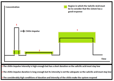
First of all, it is necesary to define the desired response, in this case the Salicylic Acid. Thus, we stablished some ranges where concentration supposed to be. This response depends on the chitin or 3-OH-PAME impulse. Besides, the system is preferable to respond if the signal is long and intense. On the other hand, we don't want our cells to be "awake". The figure below shows this:
- Step 2. Optimization of parameters: A point within an area
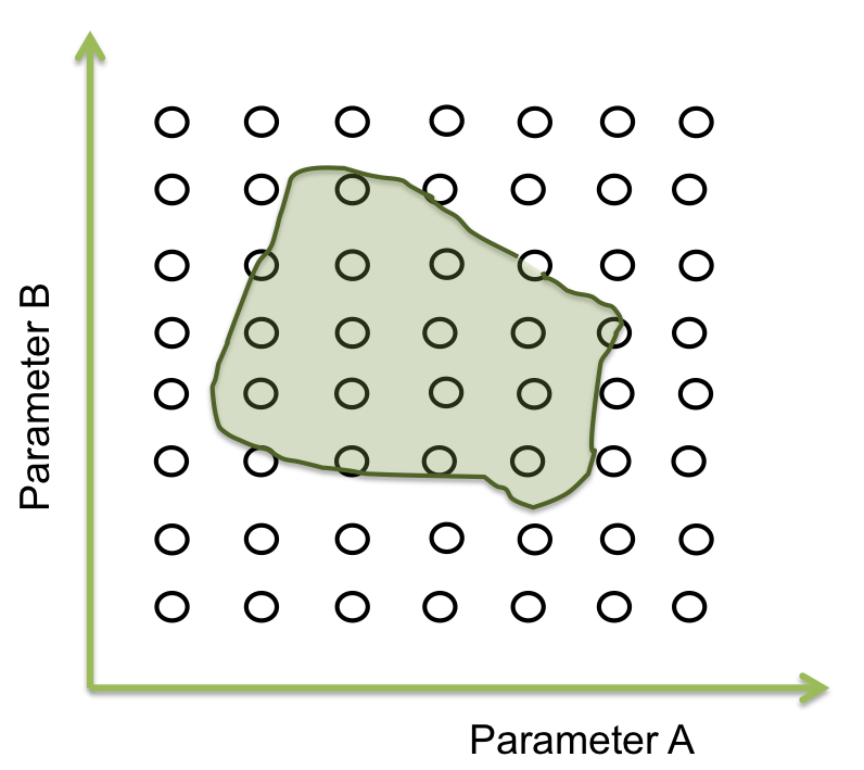
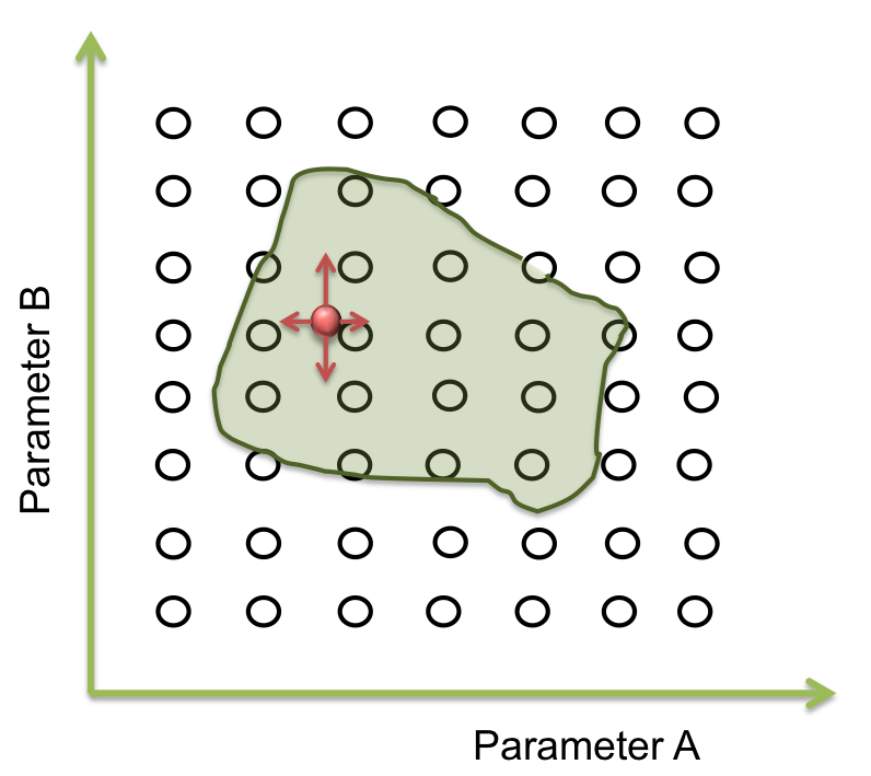
Within the parameter space, there are many sets of them that make the system behaves just like expected; and these can be represented as an area. The main objective is to find this area. Suppose you only have two parameters. The plane represents the parameter space and the green area is where the system works.
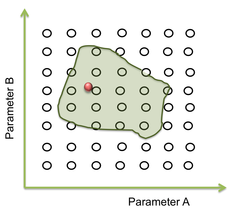
Now we want a point within these area to begin the screening. It seems easy to identify in two dimensions, but this process can take a lot of time (weeks or even months) when it is a space of more than 10 parameters. So, one way to achieve this process is making an optimization.
A process of optimization takes a function and found maximum or minimum values changing some variables of it. The changing variables are named optimization variables and function is called objective function. If we have some limitations, it is possible to add restrictions to the system, and the function will be optimized without breaking them.
In this case, the objective function is a minimum difference of squares between the points of the expected behavior and the response of the equations with a set of optimization variables. When the distance between these points is minimum, the parameters are found.
This optimization process was done discretizing the differential equations and putting them as restrictions. The same procedure was made for the stable state concentration where the differential equation must be equal to zero (when there is no signal). This algorithm was programmed in a specialized software.
Unfortunately the firsts results were not satisfactory and a new code it is being developed.
- Step 3: Sensitivity anlysis
In this step the importance of each parameters in the main outputs behavior (Our case: Salicylic Acid, the toxin HipA7 and the antitoxin HipB) is tested. The objective is to find how much each parameter affect the desired response.
This test considered the following stages: i.) Establish the ranges of the parameters (see above), ii) Determine appropriate division for the ranges, iii) Iterate each parameter while leaving the others fixed in the MATLAB code. iv) See how the difference between the steady state's concentrations and the concentrations during the impulse of the pathogen changed with the change of each parameter.
Note: the exact value for each parameter is not important. It is important their relevance and how they change the response.
Here is an example:
The figure above shows how the HipB, HipA7 and Salicylic Acid concentration change during the presence of the pathogen is significantly influenced by the maximal production rate of LuxI protein. We make this procedure for all the parameters in both systems (Ralstonia and Fungus). The results are shown below:
Fungus:
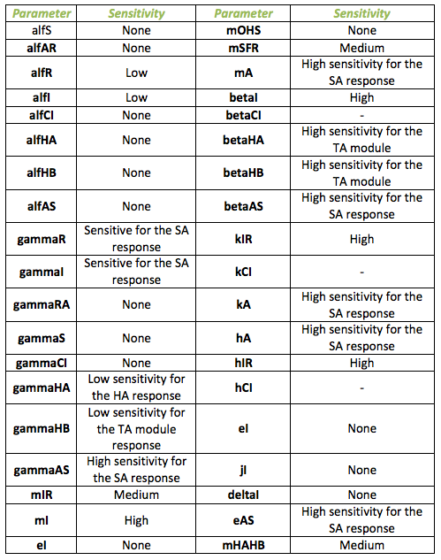
The sensitivity analysis was performed for the system with the fungal detection module. The following table shows the different parameters involved in the system with the fungal detection module. Besides, it shows how they affect the final behavior.
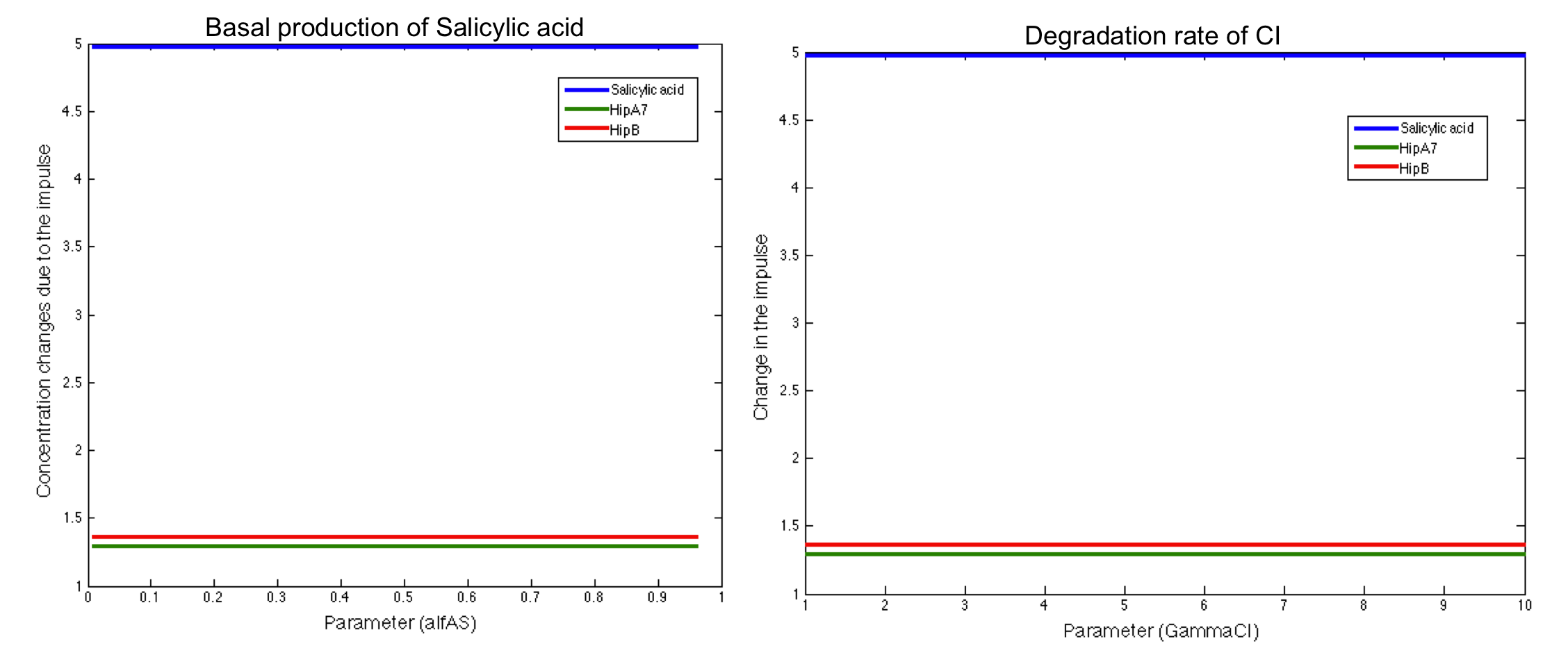
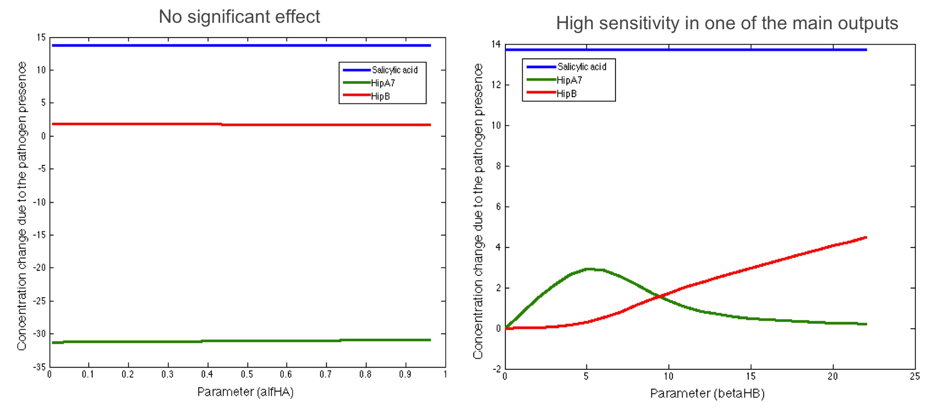
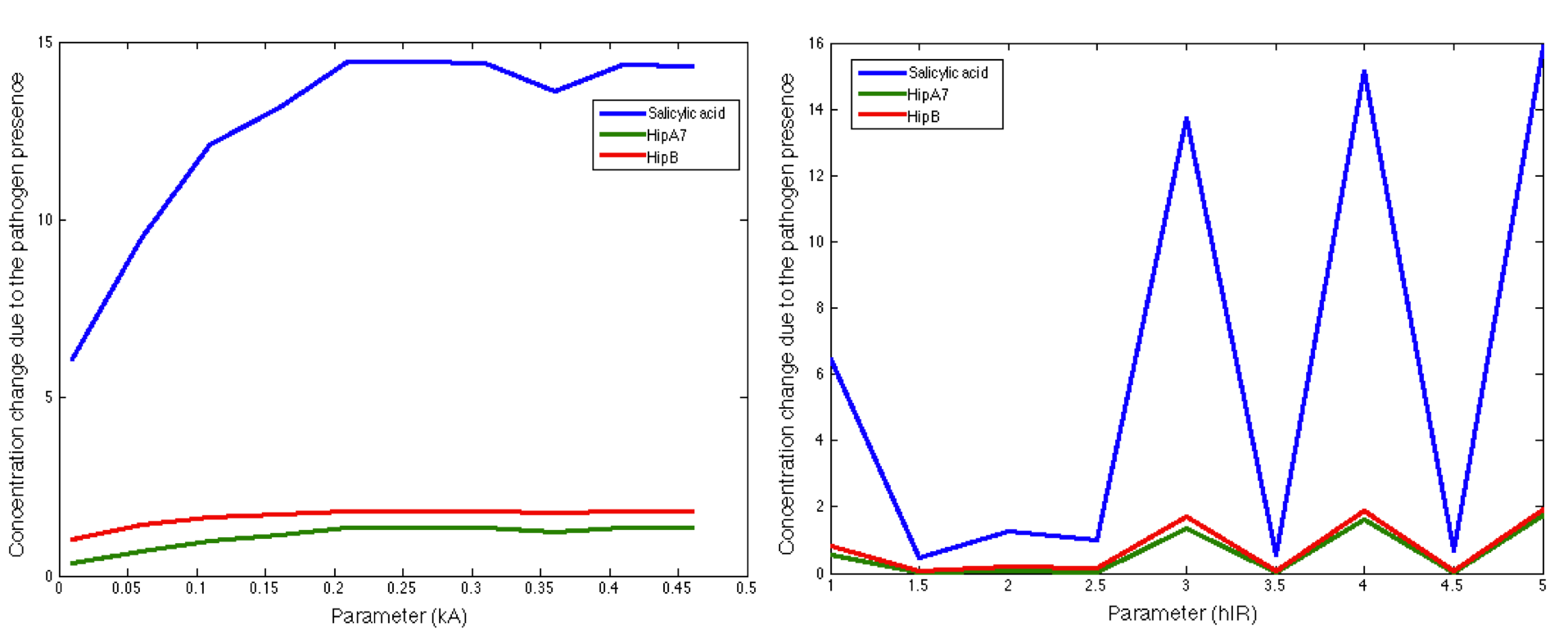
Here we present some of the graphics found in the analysis. The figures below show two parameters that do not have significant influence in the desired response:
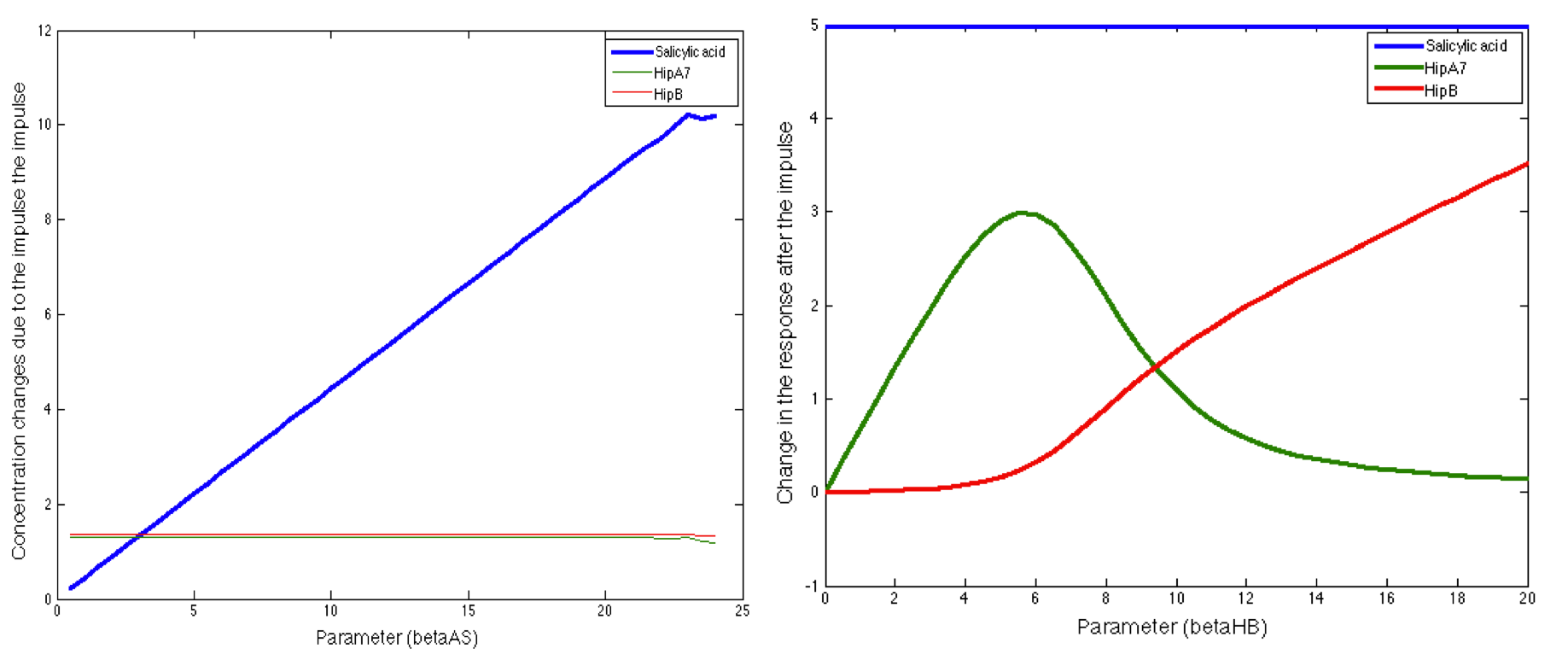
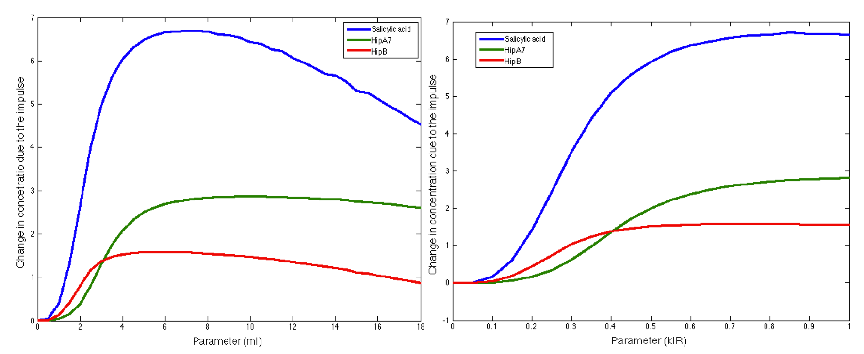
We also found some parameters that have a significant influence in one of the main outputs but were not sensitive to the rest:
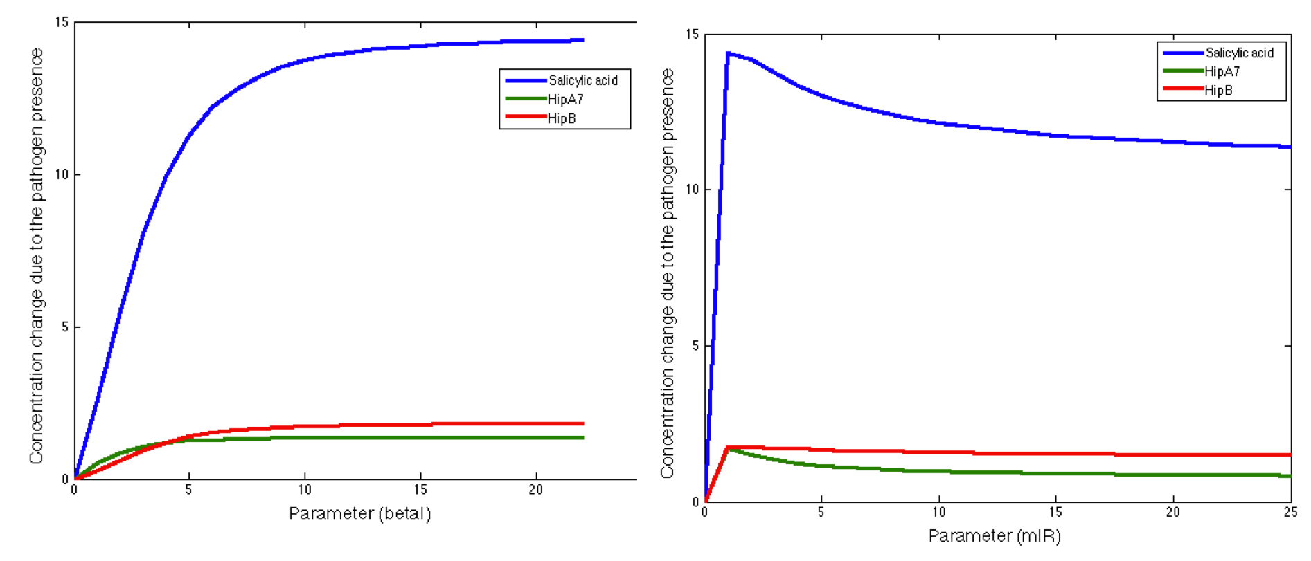
Finally, we found some parameters that affect the final response of all the main outputs of interest:
Ralstonia
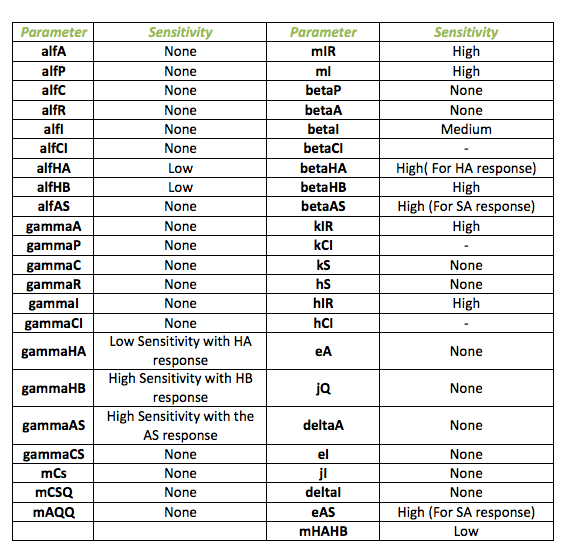
Below, it is exposed the results obtained from sensitivity test for Ralstonia. The next table identifies those parameters that make a relevant change in the model from those that do not. The main outputs tested were the HipB, HipA7 and the salicylic acid change in concentration due to the impulse.
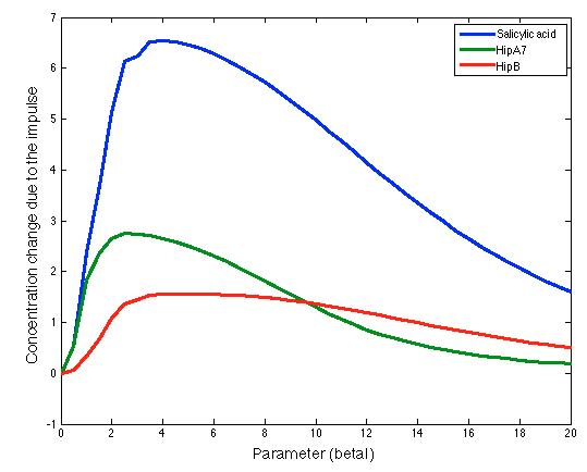
The following figures show the results obtained for almost all the relevant parameters. Like in the previous case we found some parameters that had no effect at all in the response and others than only had effect in one of the main outputs.
We also found some interesting results, there were some parameters that had a significant influence in a small range, but when the rest of the range was evaluated the response was not sensitive to these parameters:
Finally we found parameters that had significant influence in the response of the three main outputs and in the complete range of the parameter. Here we present some of the most interesting behaviors of these kind of parameters:
Using this results it is possible to know the parameters that affect the response in a major way. Although it is still unknown the exact value of the parameter, it is possible predict how the system is supposed to response. Then, we could proceed to the final step.
- Step 4: Screening
- If we have a set of parameters, why do we do a screening?
In the second step we found a set of parameters that give the expected response of the system. But this is only a point. What does happen with the rest of points of the area? Does the optimization method “know” if these parameters are real or have biological sense? As long as we specified one single response for the parameters, we don’t know if there are other possible responses of valid solutions. Do they exist?
To answer these questions we performed a screening of the parameters. Beginning at the resulting point of the optimization, we started to move in all directions in a fixed range and then we examined when the acceptable area ends.
How much do we move depends on the sensitivity analysis. If the response is not very sensitive to the parameter, we take longer steps than the case which the response is more sensitive.
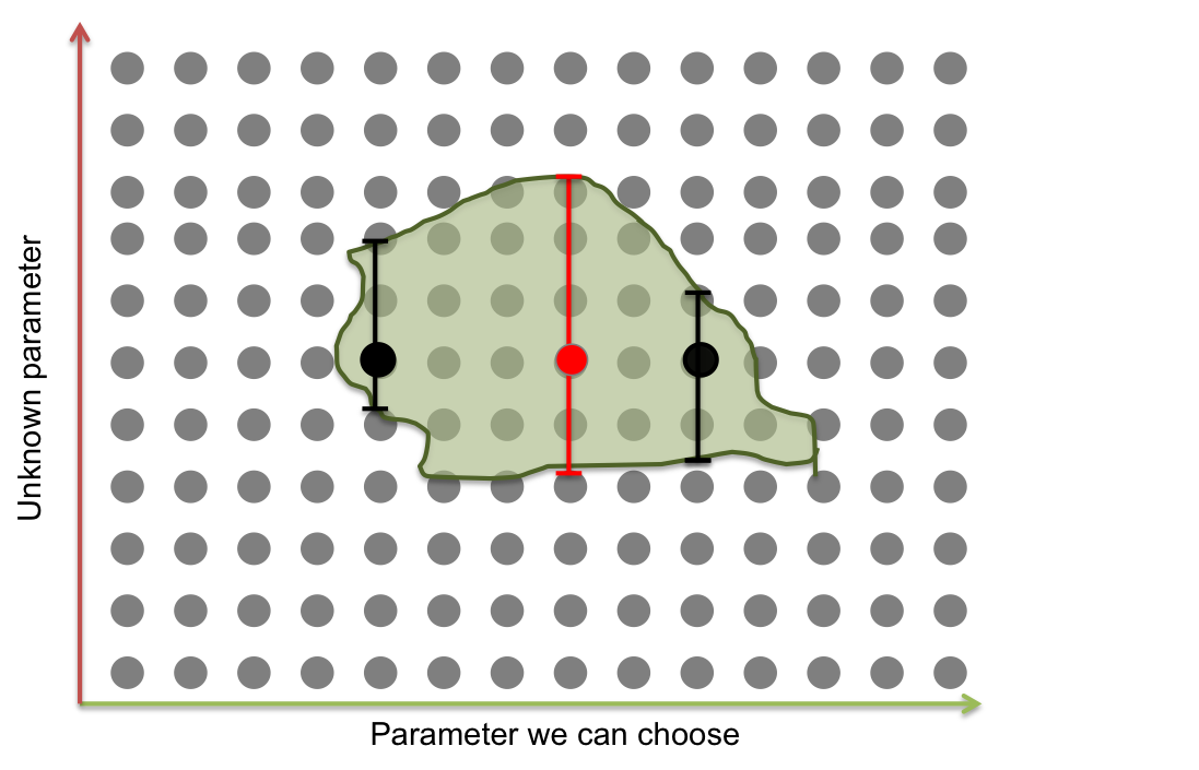
There are some parameters that can me modified experimentally like the maximal rate production but most of them depend on molecular details, are unchangeable and can only be known with experiments. The final goal of these standard procedure is to set the changeable parameters in such a way that the cross sectional area of the area of parameters that has desired response is maximized.
Suppose you only have two parameters, one that can be changed and one that does not. If you set the first parameter in a black dot (see figure below), a small change of the uncontrollable parameter would take the system out of its working area. The optimum solution is to set the first parameter in the red line, so the probability of going out of the working area is smaller.
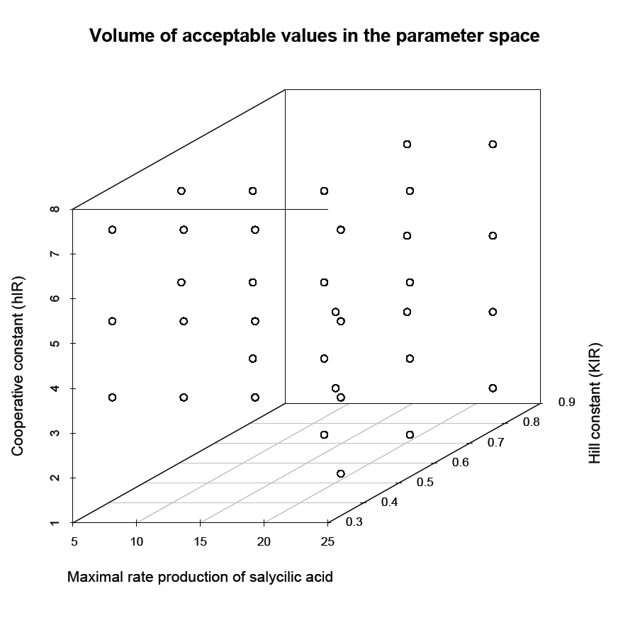
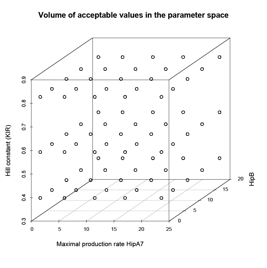
In the first trial we got this results
We made a screening with very few steps because of the little computational time, which results are shown on section 4. At this moment we are running a screening with more steps in order to make it more precise.
 "
"

