Team:SJTU-BioX-Shanghai/Project/project3
From 2012.igem.org
(→Diffusion Model) |
Huanan1991 (Talk | contribs) (→Basic Assumptions) |
||
| (19 intermediate revisions not shown) | |||
| Line 24: | Line 24: | ||
<td valign="top" width="750"> | <td valign="top" width="750"> | ||
__NOTOC__ | __NOTOC__ | ||
| + | =Acceleration Modeling= | ||
| + | {{Template:12SJTU_part_summary_head}} | ||
| - | + | *'''State of Art''' | |
| - | + | ||
In mathematics, a partial differential equation (PDE) is a differential equation that contains unknown multivariable functions and their partial derivatives. PDEs are used to formulate problems involving functions of several variables, and are either solved by hand, or used to create a relevant computer model. | In mathematics, a partial differential equation (PDE) is a differential equation that contains unknown multivariable functions and their partial derivatives. PDEs are used to formulate problems involving functions of several variables, and are either solved by hand, or used to create a relevant computer model. | ||
| + | |||
| + | Mathematical modeling is a useful tool for understanding how a bio-system works and how to improve it. We build a mathematical model mainly based on the mechanism of the involved biochemical reaction. Here we focus on the dynamic process of membrane protein cluster in order to reveal how the system works over time. | ||
| + | *'''Aim''' | ||
PDEs can be used to describe a wide variety of phenomena such as sound, heat, electrostatics, electrodynamics, fluid flow, or elasticity. Defined by the PDE, the variable describing the phenomena can be solved according to different boundary values. | PDEs can be used to describe a wide variety of phenomena such as sound, heat, electrostatics, electrodynamics, fluid flow, or elasticity. Defined by the PDE, the variable describing the phenomena can be solved according to different boundary values. | ||
| - | + | *'''Achievements''' | |
| + | |||
| + | Based on diffusion equation, by solving it under different boundary values, we found that the cluster system can increase production significantly. | ||
| + | {{Template:12SJTU_part_summary_foot}} | ||
| + | ==Basic Assumptions== | ||
| - | :1. | + | :1. Protein clusters locate on the membrane, which means the products of our device diffuse in an area of hemisphere. We assume that the membrane has no extra effect on the behavior of molecular diffusion. So the concentration will be doubled compared to the diffusion progress in a volume of sphere. |
| - | :2. The | + | :2. The primary substrate concentration remains the same in the cell cytoplasm. |
:3. The products of our cluster enzyme diffuse as the diffusion equation. The diffusion equation is a partial differential equation which describes density dynamics in a material undergoing diffusion. It is also used to describe processes exhibiting diffusive-like behavior, which means the diffusion rate is proportional to the gradient of density. | :3. The products of our cluster enzyme diffuse as the diffusion equation. The diffusion equation is a partial differential equation which describes density dynamics in a material undergoing diffusion. It is also used to describe processes exhibiting diffusive-like behavior, which means the diffusion rate is proportional to the gradient of density. | ||
:4. Each our membrane device occupies an area of membrane, adjacent to the others. Because each device is the same as others, the diffusion of the products out of the area can be regarded as reflected by the imaginary barrier, which means the normal derivative at the edge of the area is 0. | :4. Each our membrane device occupies an area of membrane, adjacent to the others. Because each device is the same as others, the diffusion of the products out of the area can be regarded as reflected by the imaginary barrier, which means the normal derivative at the edge of the area is 0. | ||
:5. The enzyme can be regarded as a thermal source, producing the molecular at a rate of v. | :5. The enzyme can be regarded as a thermal source, producing the molecular at a rate of v. | ||
| - | |||
| - | |||
| - | |||
==Acceleration Model== | ==Acceleration Model== | ||
| Line 47: | Line 52: | ||
===Diffusion Model=== | ===Diffusion Model=== | ||
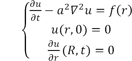
:The diffusion area is regarded as a hemisphere which radius is R with an enzyme located on the center which occupies a region of r<sub>0</sub>. So we have the equaction: | :The diffusion area is regarded as a hemisphere which radius is R with an enzyme located on the center which occupies a region of r<sub>0</sub>. So we have the equaction: | ||
| - | + | [[Image:12SJTU_formula1.png|200px]] | |
| - | : | + | |
| - | + | ||
| - | + | ||
| - | + | ||
| - | + | ||
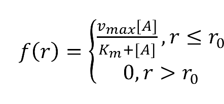
::While: | ::While: | ||
| - | + | [[Image:12SJTU_formula11.png|200px]] | |
| - | + | ||
| - | + | ||
| - | + | ||
| - | + | ||
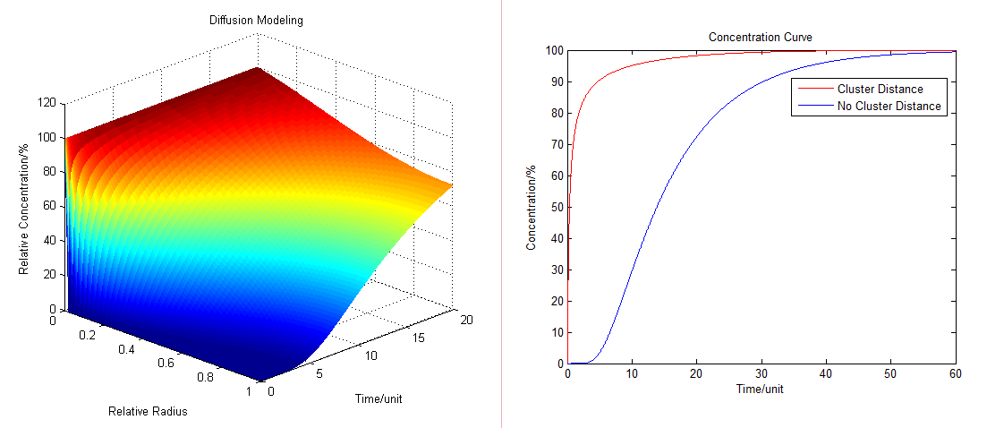
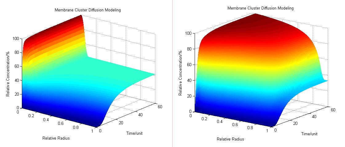
:By solving the equations we can show how the concentration floats with radius and time (''Fig.1'' ): | :By solving the equations we can show how the concentration floats with radius and time (''Fig.1'' ): | ||
| Line 69: | Line 65: | ||
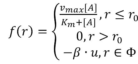
:We place another downstream enzyme beside the current enzyme, so the production will be consumed. The consumption rate is considered to be Michaelis-Menten equation, and simplified as proportional to the product concentration. | :We place another downstream enzyme beside the current enzyme, so the production will be consumed. The consumption rate is considered to be Michaelis-Menten equation, and simplified as proportional to the product concentration. | ||
| - | : | + | [[Image:12SJTU_formula1.png|200px]] |
| - | + | ||
| - | + | ||
| - | + | ||
| - | + | ||
::While: | ::While: | ||
| - | + | [[Image:12SJTU_formula12.png|200px]] | |
| - | + | ||
| - | + | ||
| - | + | ||
| - | + | ||
:Then we have three-dimensional graphics as following (''Fig.2'' ): | :Then we have three-dimensional graphics as following (''Fig.2'' ): | ||
| Line 87: | Line 75: | ||
[[Image:12SJTU_Modelling45.png|thumb|600px|center|''Fig.2'' : Membrane Cluster Diffusion Model near/far]] | [[Image:12SJTU_Modelling45.png|thumb|600px|center|''Fig.2'' : Membrane Cluster Diffusion Model near/far]] | ||
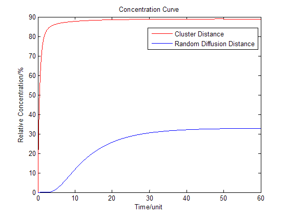
| - | :To compare the concentration at different distance we have: | + | :To compare the concentration at different distance, tracing the concentration aside the enzyme we have: |
[[Image:12SJTU_Modelling5.png|thumb|600px|center|''Fig.3'' : Comparison of concentration at different distance in Membrane Cluster Diffusion Model]] | [[Image:12SJTU_Modelling5.png|thumb|600px|center|''Fig.3'' : Comparison of concentration at different distance in Membrane Cluster Diffusion Model]] | ||
| Line 93: | Line 81: | ||
===Enzymatic Reaction with Product Inhibition=== | ===Enzymatic Reaction with Product Inhibition=== | ||
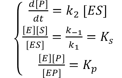
| - | + | [[Image:12SJTU_formula2.png|200px]] | |
| - | + | ||
| - | : | + | |
| - | + | ||
| - | + | ||
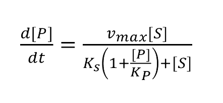
:Solving these equations we have: | :Solving these equations we have: | ||
| - | + | [[Image:12SJTU_formula21.png|250px]] | |
| - | + | ||
| - | : | + | |
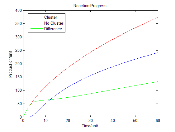
[[Image:12SJTU_Modelling6.png|thumb|500px|center|''Fig.4'' : Production in enzymatic reaction with product inhibition]] | [[Image:12SJTU_Modelling6.png|thumb|500px|center|''Fig.4'' : Production in enzymatic reaction with product inhibition]] | ||
Latest revision as of 03:58, 27 September 2012
| ||
|
 "
"
