Team:SEU O China/Model
From 2012.igem.org
| Line 142: | Line 142: | ||
Experiment Group: | Experiment Group: | ||
<img src="https://static.igem.org/mediawiki/2012/f/f2/Lightmodelexp.gif"> | <img src="https://static.igem.org/mediawiki/2012/f/f2/Lightmodelexp.gif"> | ||
| - | </center> | + | </center><br><br> |
| + | </html> | ||
| + | |||
| + | ---- | ||
| + | |||
| + | |||
| + | '''Modeling Parameters''' | ||
| + | |||
| + | |||
| + | *Recovery time: tr=2 | ||
| + | *Releasing Constant: q=600; | ||
| + | *Decomposition Constant: y=1; | ||
| + | *Diffusion Constant: D=0.15; | ||
| + | |||
| + | |||
| + | <html> | ||
<div class="clear"></div> | <div class="clear"></div> | ||
</div> | </div> | ||
| Line 212: | Line 227: | ||
<br><br><br>Experiment Group: | <br><br><br>Experiment Group: | ||
<img src="https://static.igem.org/mediawiki/2012/4/47/Macromodel2.gif"> | <img src="https://static.igem.org/mediawiki/2012/4/47/Macromodel2.gif"> | ||
| - | </center> | + | </center><br><br> |
| + | </html> | ||
| + | |||
| + | ---- | ||
| + | |||
| + | |||
| + | '''Modeling Parameters''' | ||
| + | |||
| + | |||
| + | *Releasing Constant: q=150; | ||
| + | *Decomposition Constant: y=1; | ||
| + | *Diffusion Constant: D=0.20; | ||
| + | *Cellular Movement Constant: V=1; | ||
| + | *Parameter between AHL density and Nm: a=20, b=0.5, c=0.009, d=0.01 | ||
| + | |||
| + | |||
| + | <html> | ||
<div class="clear"></div> | <div class="clear"></div> | ||
</div> | </div> | ||
| Line 271: | Line 302: | ||
<br><br><br> | <br><br><br> | ||
Experiment Group: | Experiment Group: | ||
| - | <img src="https://static.igem.org/mediawiki/2012/8/8e/Automodelexp.gif"> | + | <img src="https://static.igem.org/mediawiki/2012/8/8e/Automodelexp.gif"></center><br><br> |
| + | </html> | ||
| + | |||
| + | ---- | ||
| + | |||
| + | '''Modeling Parameters''' | ||
| + | |||
| + | |||
| + | *Recovery time: tr=2 | ||
| + | *Releasing Constant: q=600; | ||
| + | *Decomposition Constant: y=1; | ||
| + | *Diffusion Constant: D=0.15; | ||
| + | *Cellular Movement Constant: V=2; | ||
| + | *Ratio of Red Cells: 0.01 | ||
| + | |||
| + | |||
| + | <html> | ||
<div class="clear"></div> | <div class="clear"></div> | ||
</div> | </div> | ||
| Line 551: | Line 598: | ||
These days, the development of normal electronic chips has met barriers from quantum level. Moreover, the requirement for smaller and more energy-saving chips has been increasing, which makes the research on bio-logical gates more meaningful than ever. However, the problem of volume and time-delay in our design should be eliminated by applying more sophisticated algorisms for more compatible and systematic design. Anyway, the bio-logical gate design under our system is still promising and worth improving. | These days, the development of normal electronic chips has met barriers from quantum level. Moreover, the requirement for smaller and more energy-saving chips has been increasing, which makes the research on bio-logical gates more meaningful than ever. However, the problem of volume and time-delay in our design should be eliminated by applying more sophisticated algorisms for more compatible and systematic design. Anyway, the bio-logical gate design under our system is still promising and worth improving. | ||
| + | |||
| + | |||
| + | |||
| + | ---- | ||
| + | |||
| + | '''Modeling Parameters''' | ||
| + | |||
| + | Cellular Movement Constant: V=1; | ||
| + | |||
| + | Threshold Value for Output 1/0: h=20; | ||
| + | |||
| + | Releasing Constant: q=150; | ||
| + | |||
| + | Decomposition Constant: y=1; | ||
| + | |||
| + | Diffusion Constant: D=0.20; | ||
| + | |||
<html> | <html> | ||
<div class="clear"></div> | <div class="clear"></div> | ||
Revision as of 22:44, 26 September 2012


Modeling
System Simulation
Introduction
In order to verify the availability and probable effect of our design scheme, simulation mathematical models based on Cellular Automata technique have been conducted.
In catering to our past experiment scheme, we have constructed two models as follows:
- Light Sensing Model: use light to trigger the asymmetry process of the colony;
- Movement Model: use more complicated pathways to induce the break of symmetry.
A cellular automaton is in nature a finite-state machine in discrete time as well as space studied in computability theory,mathematics, physics, complexity science, theoretical biology and microstructure modeling.
This model provides a significant reference to the appraise of realistic experiments by simulating the whole pattern changing process, which consists of division, movement, death and some relevant ones.
Light Induced Micro Model
To display the simulation results directly, we have constructed a micro model based on cellular automata. Each minimum spatial unit is able to hold up at most one cell, which can be characterized by a cellular automaton; Meanwhile, another property that wonders in every minimum spatial unit is the density of AHL, which relies on the density diffusion equation. The detailed cellular automata rules would be as follows.
Basic Principles
a) Cell types
Each minimum spatial unit in this cellular automata model is able to hold up at most one cell. Cells can be divided into two types, normal cells(marked by green) and special cells(marked by red). Red cells are transferred from green cells by the trigger of light. The type of cells is denoted by ‘C’ as follows:
- Equation 1.
‘n’ represents the n th period, ‘(i, j)’ represents the location of the cell. Same below Red cells emit AHL at the rate of ‘q’ in every period.
b) Cell Division and Cellular States
Both kinds of cells are likely to divide. A mature cell possesses a division probability of Pdiv every time unit and gets two green cells after division. The newly generated cell would grow closely to the original cell and would emerge at the eight neighboring positions with equal probability. If the eight neighboring positions had been occupied, then the original cell would not be able to divide.
Consider the realistic condition where continuous cell division is impossible, so we use Φ to denote cellular states. At the very beginning Φ=1; Then with the cells growing, Φ=Φ+1 with every period; When Φ=τ, the cell would be mature enough to divide with a division probability of Pdiv during every period; After every division, the Φ(n;i,j) of the original and new cells would both change into:
- Equation 2.
However, in our system, as a signal molecule, AHL can trigger the antisense Ftsz part which can be functional as a division repressor. So Pdiv is actually a constant but a parameter proportional to the density of AHL. With several steps of calculations and experiments, the relationship between Pdiv and the density of AHL can be induced as follows:
- Equation 3.
Among it both ‘a’ and ‘b’ are unknown parameters.
c) Cell Movement
In the light sensing model, due to the big influence of light from the outer environment, cell movement has almost nothing to do with final results both in simulation or realistic experiments. As a result, we simplify the movement of cells. However, the movement of cells would no longer be negligible in the afterwards models. Further details on its rules and results to come afterwards.
d) Cell Death
In all models mentioned in this text, cell death has merely minor influence on our final results so it is neglected in all.
AHL Density Equation
AHL density can be expressed as u(r,t). Take the discrete characteristic of cellular automata into consideration, just denote it as . As a solute, AHL has the phenomenon of diffusion and decomposition. At mentioned above, red cells would spread out AHL. In conclusion, AHL complies to diffusion equation:
- Equation 4.
u: AHL density; D: diffusion constant; q: AHL releasing rate of a single triggered cell; γ describes the decomposition process of AHL; m: total number of cells.
Simulation Procedure
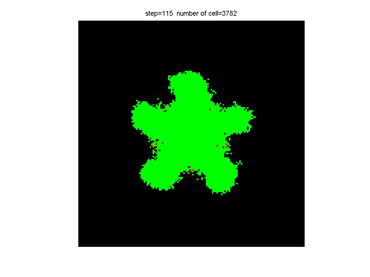
At the very beginning, AHL density u(r, 0)=0 on the infinite plane. In order to eliminate the asymmetry in the results that might be caused by the asymmetry of the original state, there is only one green cell at first. Choose several separate cells manually to shed light on. With the sliding improvement of the colony from merely one cell, green cells would eventually reach the light area where they would transform into red cells. Red cells begin to release AHL. When the quantity of red cells accumulates to a certain threshold, high density of AHL in certain areas would repress the division of cells and begin to trigger the differentiation of cell and therefore break the symmetry of the colony.
Results
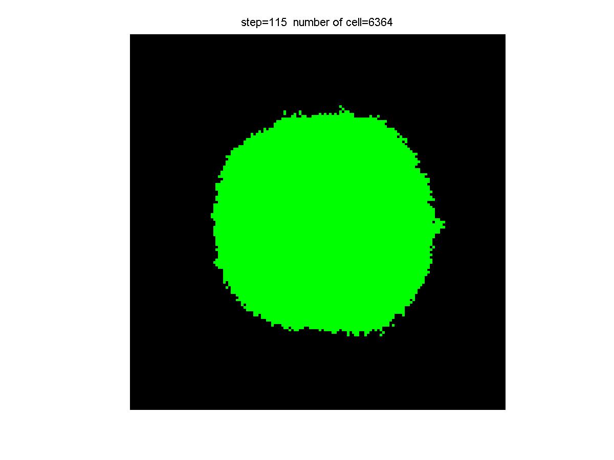
| 
|
| Control group result | Experiment group result |

Experiment Group:

Modeling Parameters
- Recovery time: tr=2
- Releasing Constant: q=600;
- Decomposition Constant: y=1;
- Diffusion Constant: D=0.15;
Light Induced Macro Model
The micro model is somehow quite easy to understand. We can relatively directly observe and analyze the location and state of each cell, so that this model is suitable for small-scale colony pattern vicissitude analysis. However the application of several random factors like division probability or others eventually complicates the anticipation process. Moreover, variations exist every time of simulation. We have to observe the shape of colony directly(with eyes) on a larger scale, which would obey the statistical rules. For the sake of seeking the most probable situation, we have a macro model to simulate. Macro model differs from the micro model mainly in that the number of cells in a spatial unit no longer limits to one but pertains to another characteristic: cellular density. The macro model would on one hand reduce the quantity of calculation and on the other hand reflects the possible results more realisticly.
Basic Principles
Compared to micro model, the AHL density u(r, t) for every spatial unit possesses the same meaning and remain compliant to equation(4). Whereas, the characteristic of cells is no longer weighed by whether existed or not, nor does the type or state of a single cell be considered, but using the density of green normal cells and that of red special cells
a) The Cellular Density Logistic Model
In the micro model, we can discuss the division process and growing period of single cells, but not in the macro model any more. For the concept of single cells is eliminated and instead we just take into consideration the quantity of cells in certain areas which would obey some kinds of rules. Here, we applied the classic Logistic Model to lineate the quantity visisitude of colony. With the original number of cells ranging from 1 and 200 and a environmental limit of 100, the changing situation of the number of cells is shown as below:
- Logistic model with initial cell number of 1 and 200
The equation is shown as follows:
- Equation 5.
Among which, k is a proportion constant, Nm denotes the environmental cell volume at the location r and time t and is a function of the AHL density u(r, t); N(r, t) denotes the number of cells at the location r and time t.
Logistic Model is a somehow realistic model which takes not only the growth of number but also the environmental tension after the growing of the number into consideration and therefore makes it more practical than the miro model.
As high AHL density would repress cell division, we can regard the environmental volume as a function of AHL density. AHL density gets higher and environmental volume Nm gets lower. The relationship might be as follows:
- Equation 6.
Among which both 'd' and 'e' are unknown parameters,and d>0.
After the change of cellular numbers, due to the background that red special cells can only be transformed by light, all newly-built cells in this Logistic Model would be green cells.
b) Cell Movement
As the movement of green cells is random movement, therefore the movement of green normal cells relies on the formula below:
Among which 'V' denotes the diffusion constant or a reflection of cellular rate.
The movement of red cells is the same.
Other parts and simulation principles of macro model are just the same with the micro model.
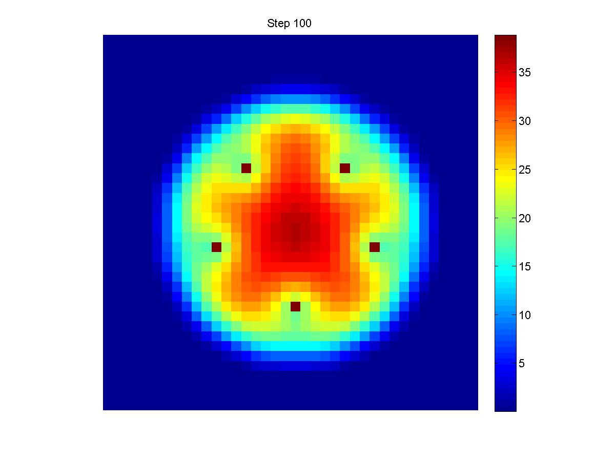
Results
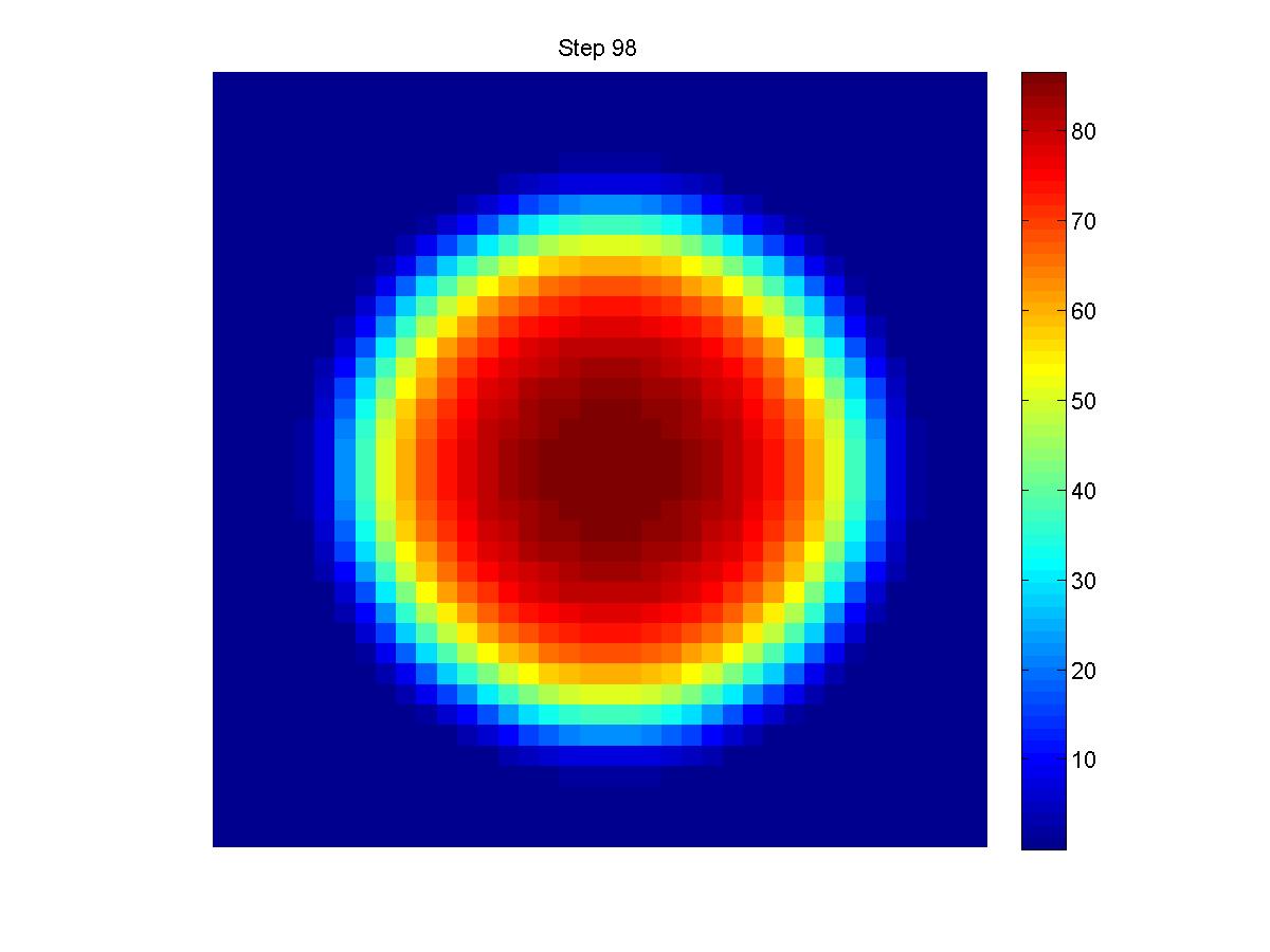
| 
|
| Control group result | Experiment group result |

Experiment Group:

Modeling Parameters
- Releasing Constant: q=150;
- Decomposition Constant: y=1;
- Diffusion Constant: D=0.20;
- Cellular Movement Constant: V=1;
- Parameter between AHL density and Nm: a=20, b=0.5, c=0.009, d=0.01
Auto-differentiation
As the light sensing model requires outer signal to trigger the break of symmetry, this is not a rather ideal condition. Therefore we manage to realize the break of symmetry with more complicated pathways.
Basic Principles
The basis of auto-differentiation model is cellular automata, which includes a number of same rules as the micro model. But the most obvious difference lies in that the red special cells are not triggered by light stimulus any more but rely on a constant probability of during every division period. Under this circumstance, the locations of red cells are discrete and unstable and as a result, the movement of red cells requires consideration.
a) Cell Movement
Red special cells tend to move to high AHL density areas. The tendency would be as follows: Red cells originally move in random directions and at a rate of vr; Red cells have two movement tendencies, turning to a direction or moving along. Every step of movement generates a density gap of Δu and this value would be determinant to the choice of turning around or moving along. Lower density gap would lead to higher probability of turning around. And therefore:
- Equation 7.
Among which, 'f' and 'g' are unknown parameters.
Green cells still comply to the rule of random movement.
b) Cell Division So long as in the auto-differentiation model, red special cells are generated by cell division, the newly-built cell would own a probability of Pred to become red and a probability of 1-Pred to become green. The original cell would stay in its previous state. The ration of red/green would remain almost constant by this method.
The other rules, such as the diffusion of AHL molecules, are the same as the light induced mode.
Simulation Process
The original state would be the same as the micro model where the AHL density u(r, 0)=0 on the infinite plane. Several red special and green cells are randomly distributed in a rather tiny area.
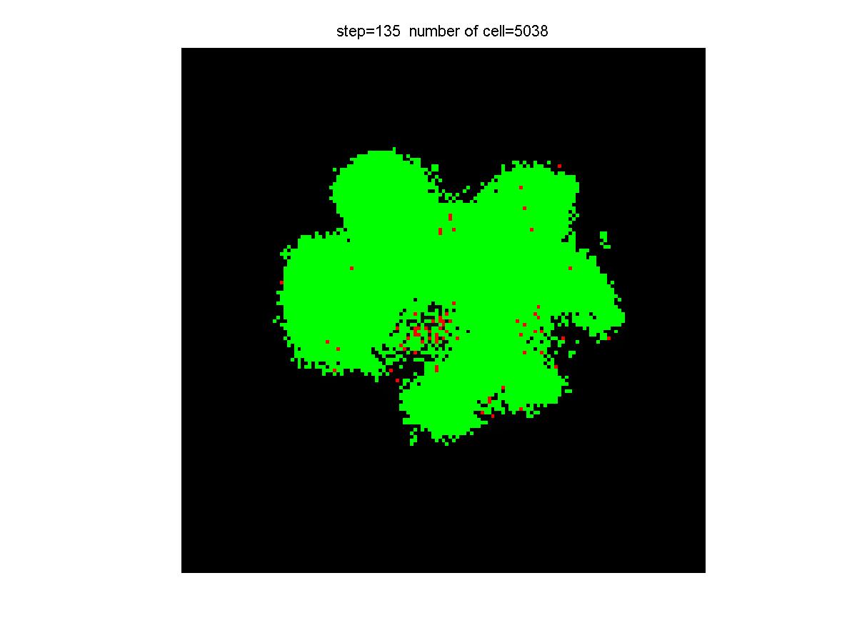
After the simulation has begun, the size of colony slowly increases with cell division and movement. Red cells would release AHL and at the same time tend to move to high density areas and lead to the appearance of several piles of red cells, around which AHL density is high enough to repress cell division. With the different division rate of cells (mainly green cells), the symmetry would be broken and the colony would turn into different patterns.
The final shape of colony is mainly controlled by the clustering phenomenon of red cells. And as this clustering phenomenon can be influenced by a number of random factors, the eventual colony is unlikely to be symmetry. Meanwhile, there has not existed an appropriate method to analyze the clustering behavior, which means the final shape in the movement model cannot be controlled accurately yet.
Results
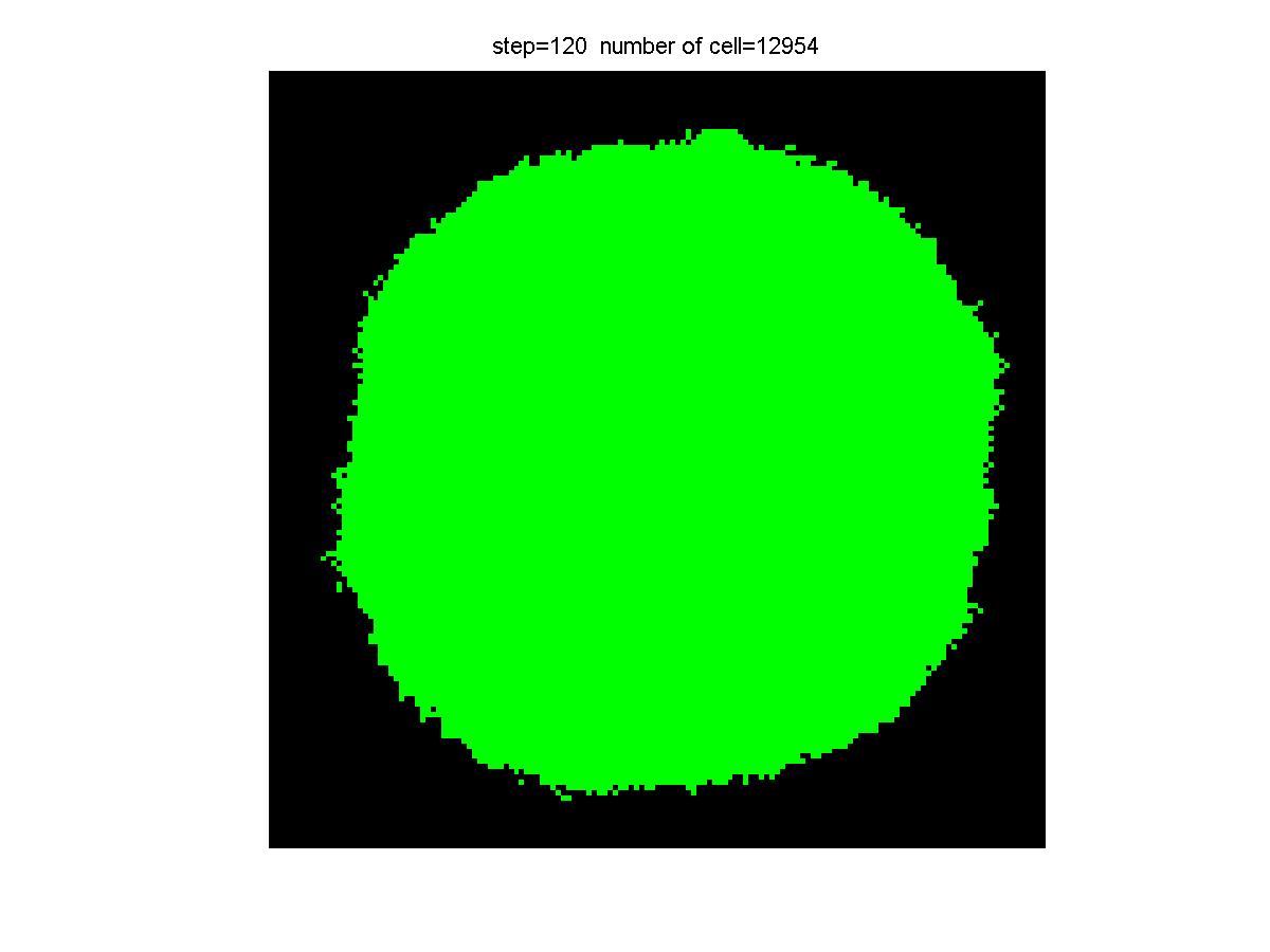
| 
|
| Control group result | Experiment group result |

Experiment Group:

Modeling Parameters
- Recovery time: tr=2
- Releasing Constant: q=600;
- Decomposition Constant: y=1;
- Diffusion Constant: D=0.15;
- Cellular Movement Constant: V=2;
- Ratio of Red Cells: 0.01
Parameter Estimation
Introduction
To build a biobrick building, it is important to make sure each part of the building can work as expected. Sometimes, what we concern is not only a part is right or wrong, but precisely how it works. What is the generating rate of a molecule? How can we describe the efficiency of a asRNA silencing? Quantifying the experiment data, parameter estimation is a vital step when we try to combine project design, mathematical modeling and biological experiment.
Here, we are going to introduce an approximate Bayesian computation method for parameter inference in gene expression model, and perform a little test on our experiment data.
Approximate Bayesian computation (ABC)
ABC methods have been conceived with the aim of inferring posterior distribution where likelihood functions are computationally intractable or too costly to evaluate. They exploit the computational efficiency of model simulation techniques by replacing the calculation of the likelihood with a comparison between the observed and simulated data.
Let θ be a parameter vector to be estimated. Given the prior distribution &pi(θ), the goal is to approximate the posterior distribution,
where f(x|θ) is the likelihood ofθgiven the data x. The output of an ABC algorithm is a sample of parameters from a distribution
(D,D' is observed data and stimulated data respectively, ρ(D,D') is a kind of distance, εis a tolerance). If ε is sufficiently small, then the distribution
will be a good approximation for the posterior distribution
The simplest ABC algorithm is the ABC rejection sampler (Pritchard et al.1999), which is as follow
- Generate θ* from &pi(θ)
- Simulate D' from model M with parameterθ
- Calculate a measure of distance ρ(D,D') between D’ and D
- Accept θ if ρ<ε, and return 1.
The disadvantage of the ABC rejection sampler is that the acceptance rate is low when the prior distribution is very different from the posterior distribution. To avoid this problem, an ABC method based on Markov chain Monte Carlo was introduced (Marjoram et al.2003). The ABC MCMC algorithm proceeds as follows:
- If at θ propose a move to θ’ according to a transition kernel q(θ->θ’)
- Generate D’ using model M with parameters θ’
- If ρ(D,D’)<=ε, go to 4, and otherwise stay at θ and return 1
- Calculate: File:Seuofun12.GIF
- Move to θ’ with probability h, else stay at θ.
Gene expression model
This part concerns the posterior distribution of parameter in gene expression model via approximate Bayesian computation.
In this model, the relationship of the concentration of gene, mRNA, protein can be represented the following differential equations:
r: concentration of mRNA. p: concentration of protein. V: degradation rate of mRNA. U: degradation rate of protein. C: gene transcription coefficient. L: mRNA translation coefficient.
Here, we take the vector (U, V) as (0.05, 0.5), and obtain the posterior distribution of C and L respectively.
The data {rd[i],pd[i]} are noisy observations of the stimulated gene expression model with parameter values set at (C, L) = (1, 1). We sample nine data points (for mRNA and protein) from the solution of the system for parameter (U, V) = (0.05, 0.5) and add Gaussian noise N(0,0.03^2) (figure 1). Let the distance function d((rd,pd),(r,p)), between the data {rd[i],pd[i]}, i=1,2,…,10 , and a simulated solution for proposed parameters, {r [i],p [i]}, be the sum of squared errors.
The distance between our noisy data and the deterministic solution for (C, L) = (1, 1) from which the data were generated is 1.5. The prior distributions for C and L are taken to be uniform, C, L~U (-5, 5). The inferred posterior distributions are shown in figure 2.
- Figure 1: Trajectory of mRNA (solid curve) and protein (dashed curve) concentrations of gene expression model and the data points (circles, mRNA data; asterisks, protein) data).
- Figure 2 Parameters inferred by the ABC MCMC
Actually, there is a time delay in gene transcription and translation, so we can improve gene expression model as follows:
α,β: the time delay in gene transcription and translation. With the (α,β)=(1,1), a new result can be acquired following the previous solution.
We also sample nine data points from the solution of the system for parameter (U, V) = (0.05, 0.5) and add Gaussian noise N(0,0.3^2). (figure 3)
- Figure 3: Trajectory of mRNA (solid curve) and protein (dashed curve) concentrations of gene expression model and the data points (circles, mRNA data; asterisks, protein) data) considering time delay in gene transcription and translation.
The new inferred posterior distributions are shown in figure 4.
- Figure 4 Parameters inferred by the ABC MCMC considering time delay in gene transcription and translation.
References
Pritchard,J.,Seielstad,M.T.,Perez-Lezaun,A.&Feldman,M.W.1999 Population growth of human Y chromosomes: a study of Y chromosome microsatellites. Mol. Biol.Evo.16, 1791-1798.
Marjoram, P.,Molitor,J., Plagnol, V.&Tavare,S.2003 Markov chain Monte Carlo without likelihoods. Proc.Natl Acad. Sci. USA 100,15 324-15 328.
Experiment Data
To show the how the ABC method work, here we take the TBY experiment data as an example.
Image Process
In order to transform the experiment photograph into quantified data, we write a simple image processing program.
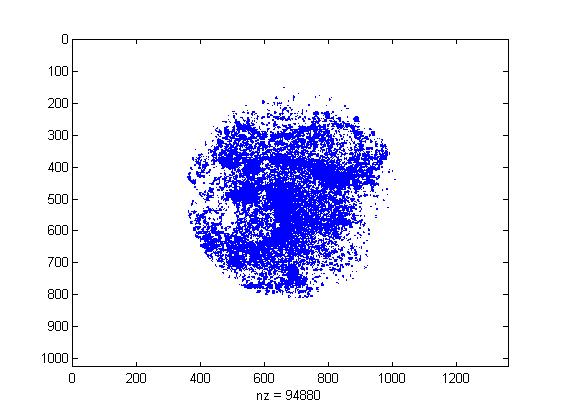
The program firstly determine the region of culture dish, and then extract the points of high brightness, which is the bacteria colony. By calculating the rate of total colony area and culture dish area, we get the colony covering rate.
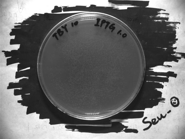
- The original photograph
- The colony pattern extracted by our program. The colony covering rate is 0.2774. For more data, see the result page.
Regression
With the all the colony covering rate data, we can calculate out the relationship between colony covering rate, which represent the expression rate of FtsZ, and the density of IPTG, which directly related to the expression of antisense FtsZ mRNA. To match then experiment data and real biology process, we choose the function R=a*exp(b*IPTG(mM))
- Regression map of colony covering rate and IPTG density. The function is R1=74.09*exp(-0.88*IPTG(mM))
Distribution
Using the regression parameter as input, we can get the posterior distributions of unknown parameters through the ABC model.
- Posterior distribution of parameter b.
Disscussion
It seems that the ABC method is unnecessary in this situation, since with the regressed function and a F-test, we can easily accept a certain parameter. So, why should we use ABC?
First, in most biological process, the distribution of a parameter is unknown. There is a high risk when we simply suggest that the parameter has a F-distribution. But with the ABC method, we can actually calculate the distribution out, which enable us to look deep into the mechanism behind the single parameter.
In addition, while building a large system with several related parts, the ABC method would become more important. There is always an error when we use a single parameter to determine the system efficiency. With the system growing up, a part linking to another, the error will be larger and larger during the iteration of part connection, but we do not even know about it sometimes. For example, a parameter of part A is 1.0 with a 0.95 certainty, and another parameter of part B is 2.0 with a 0.9 certainty. When we connect the two parts together, most times we simply combine the two functions together, and get a parameter. However, though the parameter may still be right, the confidence of it is much lower.
This problem may never happen in the ABC method, because instead of a single parameter, we can always get a posterior distribution. Thus, we can see the span of the distribution while combining the systems together, and try to control it through the process.
Bio-Computer
Our Idea
Founding on our existed system, we appoint the light signal provided in specific positions as an input and density of cells in certain points as an output.
Feasibility Analysis
For such a bio-computing system, every cell stores and transfers its state under the control of neighboring signal. This would allow for a construction of a cellular automata system on a biological level. Though only a simple logical gate presented here, an infinite memory space could be assumed and such an equivalent Turing Machine would make almost any further complicated calculation at least theoretically possible.
Advantage
The density of cells in certain points can be measured by light absorbtion, which would use light both as input and output, making it easy to execute. Meanwhile, combinations of several levels of logical gates would be available in rather tiny areas (even single colony).
Realization
See the colony a n-in, 1-out system. Use Boolean algebra parameter 1/0 to denote the existence or nonexistence of light in N input points of r1, r2, … to rn . The output is determined by whether the cellular density is larger than a threshold value of h. If it is larger than 1 then the output equals 1, otherwise the output equals 0. The output results can be judged by eyes or more professional instruments such as spectrophotometers.
Results
One dimension model for a 2-Input NAND Gate
- Light Input Location: 35, 45.
- Cellular Density Output Location: 40.
- File:Seuomodequ1.GIF
- Truth Table:
| A | B | L | Result |
| 0 | 0 | 1 | 450px |
| 1 | 0 | 1 | 450px |
| 1 | 1 | 0 | 450px |
One dimension model for a 2-Input NOR Gate
- Light Input Location: 38, 42.
- Cellular Density Output Location: 40.
- File:Seuomodequ2.GIF
- Truth Table:
| A | B | L | Result |
| 0 | 0 | 1 | 450px |
| 0 | 1 | 0 | 450px |
| 1 | 1 | 0 | 450px |
Two dimension model for a 4-Input NAND Gate
- Light Input Location: A(31,40), B(49,40), C(40,31), D(40,49).
- Cellular Density Output Location: (40,40).(Shown below)
- File:Seuomodequ3.GIF
- Truth Table:
| A | B | C | D | L | Result | Density |
| 0 | 0 | 0 | 0 | 1 | 400px | 54.9100 |
| 0 | 0 | 1 | 0 | 1 | 399px | 41.2043 |
| 0 | 0 | 1 | 1 | 1 | 400px | 29.6017 |
| 1 | 0 | 1 | 1 | 1 | 400px | 21.2919 |
| 1 | 1 | 1 | 1 | 0 | 400px | 16.2095 |
Two dimension model for a 4-Input NOR Gate
- Light Input Location: A(37,40), B(43,40), C(40,37), D(40,43).
- Cellular Density Output Location: (40,40).(Shown below)
- File:Seuomodequ4.GIF
- Truth Table:
| A | B | C | D | L | Result | Density |
| 0 | 0 | 0 | 0 | 1 | 400px | 54.9100 |
| 0 | 0 | 1 | 0 | 0 | 400px | 18.2540 |
| 0 | 0 | 1 | 1 | 0 | 400px | 8.5590 |
| 1 | 0 | 1 | 1 | 0 | 400px | 6.1014 |
| 1 | 1 | 1 | 1 | 0 | 400px | 4.4611 |
Summary
Dating back to even 1990s, the potential of bio-computing has already been agreed on by scientists. For this 6th generation of neuron computer, bio-logical gates are highly likely to be the fundamental unit of it. Though somehow naïve compared to electronic logical gates, we can see from our model the possibility of constructing more reliable bio-logical gates. The density of cells in certain points can be measured by light digesting, which would use light both as input and output, making it easy to execute. Meanwhile, combinations of several levels of logical gates would be available in rather tiny areas (even single colony). It has shown satisfying results under the cascaded condition.
These days, the development of normal electronic chips has met barriers from quantum level. Moreover, the requirement for smaller and more energy-saving chips has been increasing, which makes the research on bio-logical gates more meaningful than ever. However, the problem of volume and time-delay in our design should be eliminated by applying more sophisticated algorisms for more compatible and systematic design. Anyway, the bio-logical gate design under our system is still promising and worth improving.
Modeling Parameters
Cellular Movement Constant: V=1;
Threshold Value for Output 1/0: h=20;
Releasing Constant: q=150;
Decomposition Constant: y=1;
Diffusion Constant: D=0.20;

 "
"
