Team:USP-UNESP-Brazil/Associative Memory/Modeling
From 2012.igem.org
| Line 40: | Line 40: | ||
with the rate $\beta$. | with the rate $\beta$. | ||
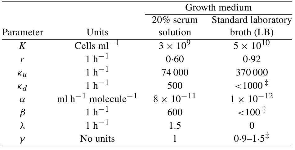
| - | {{:Team:USP-UNESP-Brazil/Templates/RImage | image=TableMatModelQS.jpeg | caption= | + | {{:Team:USP-UNESP-Brazil/Templates/RImage | image=TableMatModelQS.jpeg | caption=Table. 1. Parameter values obtained by Ward et al [1]. | size=350px}} |
| - | The authors designed some experiments in order to estimate the constants, | + | The authors designed some experiments in order to estimate the constants, Table 1. For example, the values for $K$ and $r$ were determined by examination of the growth curve. </p> |
| - | We proposed a model for two different types of population of bacteria by introducing an interaction between | + | |
| - | One population of bacteria are distinguishable of the other by the QSM that it produce. Lets call bacteria type A | + | We proposed a model for two different types of population of bacteria by introducing an interaction between them in the model proposed by Ward et al [1]. |
| + | One population of bacteria are distinguishable of the other by the QSM that it produce. Lets call bacteria type A the population that produces QSM A and the same for B. | ||
| + | The interation is represented by an aditional term in the model that makes a type A up-regulated cells becomes down-regulated by QSM B with the rate | ||
$\phi_B$ and vice-versa. | $\phi_B$ and vice-versa. | ||
\begin{align} | \begin{align} | ||
| - | \frac{d}{dt}N_{Ad} &= rN_{At}\Big[1 - \frac{N_{At}}{K}\Big] - \alpha_A A N_{Ad} + | + | \frac{d}{dt}N_{Ad} &= rN_{At}\Big[1 - \frac{N_{At}}{K}\Big] - \alpha_A A N_{Ad} + \beta_A N_{Au} + \phi_B B N_{Au} \\ |
| - | \frac{d}{dt}N_{Bd} &= rN_{Bt}\Big[1 - \frac{N_{Bt}}{K}\Big] - \alpha_B A N_{Bd} + | + | \frac{d}{dt}N_{Bd} &= rN_{Bt}\Big[1 - \frac{N_{Bt}}{K}\Big] - \alpha_B A N_{Bd} + \beta_B N_{Bu} + \phi_A A N_{Bu} \\ |
\frac{d}{dt}N_{Au} &= \alpha_A A N_{Ad} - \beta_A N_{Au} - \phi_B B N_{Au}\\ | \frac{d}{dt}N_{Au} &= \alpha_A A N_{Ad} - \beta_A N_{Au} - \phi_B B N_{Au}\\ | ||
\frac{d}{dt}N_{Bu} &= \alpha_B B N_{Bd} - \beta_B N_{Bu} - \phi_A A N_{Bu} \\ | \frac{d}{dt}N_{Bu} &= \alpha_B B N_{Bd} - \beta_B N_{Bu} - \phi_A A N_{Bu} \\ | ||
| Line 61: | Line 63: | ||
<h1 id="model">Results</h1> | <h1 id="model">Results</h1> | ||
We first evaluated the fraction of up-regulated cells as a function of the carrying capacity ($K$) and of the $\frac{\phi_A}{\phi_B}$ ratio, and $K$ turned out to be an important parameter of the model. For values of $K$ up to $10^8$, in the equilibrium, no population can reach the quorum state, since the density of cells is too low. On the other hand, for values higher than $10^8$ the population | We first evaluated the fraction of up-regulated cells as a function of the carrying capacity ($K$) and of the $\frac{\phi_A}{\phi_B}$ ratio, and $K$ turned out to be an important parameter of the model. For values of $K$ up to $10^8$, in the equilibrium, no population can reach the quorum state, since the density of cells is too low. On the other hand, for values higher than $10^8$ the population | ||
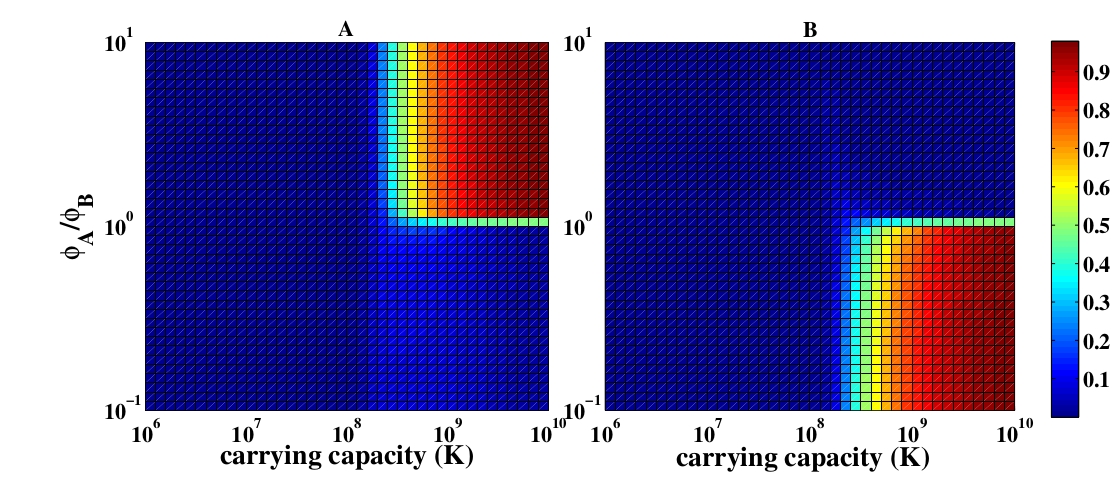
| - | that has a higher repression rate, represented by $\phi$, reaches quorum and represses the other population, as presented in Figure | + | that has a higher repression rate, represented by $\phi$, reaches quorum and represses the other population, as presented in Figure 1. |
| - | {{:Team:USP-UNESP-Brazil/Templates/RImage | image=KxRphis_alpha.jpg | caption=Fig. | + | {{:Team:USP-UNESP-Brazil/Templates/RImage | image=KxRphis_alpha.jpg | caption=Fig. 1. The fraction of the up-regulated population as a function of the carrying capacity ($K$) and the ratio $\frac{\phi_A}{\phi_B}$ for the case $\phi_B = \alpha$, at equilibrium. Initial conditions: $N_{Au} = N_{Bu} = A = B = 0$. | size=620px}} |
| - | < | + | <h2 id="model">Equilibrium points </h2> |
| - | At equilibrium we have: | + | At equilibrium point we have: |
\begin{align} | \begin{align} | ||
| Line 88: | Line 90: | ||
where $\lambda^* = \lambda/K$, and $x$ and $y$ range from 0 up to 1. These expressions are similar, since exchanging $A$ and $B$ turns one equation into the other. | where $\lambda^* = \lambda/K$, and $x$ and $y$ range from 0 up to 1. These expressions are similar, since exchanging $A$ and $B$ turns one equation into the other. | ||
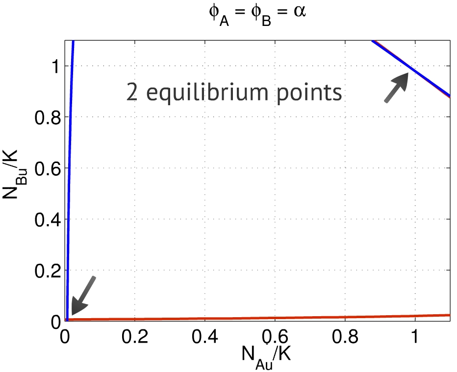
| - | {{:Team:USP-UNESP-Brazil/Templates/RImage | image=Phisiguais1.jpg | caption=Fig. | + | {{:Team:USP-UNESP-Brazil/Templates/RImage | image=Phisiguais1.jpg | caption=Fig. 2. Each curve represents the solution of one equation, their intersections being the equilibrium points. One is close to $(0,0)$, the other to $(1,1)$. | size=350px}} |
| - | Thus, the equilibrium points $(x,y)$ are placed in the intersection between the solutions for the relations above. Depending on the set of parameters, one can find two to four equilibria - the first one close to $(0,0)$, representing the repression of both populations, and the second one close to $(1,1)$, representing the activation of both populations, as presented | + | Thus, the equilibrium points $(x,y)$ are placed in the intersection between the solutions for the relations above. Depending on the set of parameters, one can find two to four equilibria - the first one close to $(0,0)$, representing the repression of both populations, and the second one close to $(1,1)$, representing the activation of both populations, as presented in Fig. 2. In this case we used the parameters presented in Table 1, for 20% serum solution growth medium. The same behavior was found using the parameters for LB growth medium. |
| Line 99: | Line 101: | ||
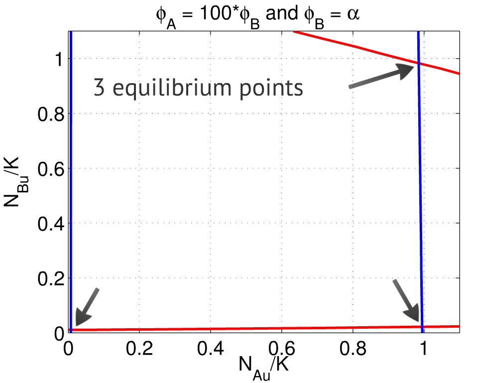
| - | {{:Team:USP-UNESP-Brazil/Templates/RImage | image=Phis100.jpg | caption=Fig. | + | {{:Team:USP-UNESP-Brazil/Templates/RImage | image=Phis100.jpg | caption=Fig. 3. When $\frac{\phi_A}{\phi_B} \gg 1$, besides the equilibria close to $(0,0)$ and $(1,1)$, there is also a point close to to $(1,0)$. | size=350px}} |
| - | A third equilibrium point emerges when $\frac{\phi_A}{\phi_B} \gg 1$ - which means the repression of population A over population B is much greater than its counterpart. In this case, the system reaches an equilibrium close to $(1,0)$: population A activated, population B repressed. The behavior is analogous if $\frac{\phi_A}{\phi_B} \ll 1$. | + | A third equilibrium point emerges when $\frac{\phi_A}{\phi_B} \gg 1$ - which means the repression of population A over population B is much greater than its counterpart, Fig. 3. In this case, the system reaches an equilibrium close to $(1,0)$: population A activated, population B repressed. The behavior is analogous if $\frac{\phi_A}{\phi_B} \ll 1$. |
| Line 115: | Line 117: | ||
Finally, when both $\phi_A$ and $\phi_B$ are big when compared to $\alpha_A$ and $\alpha_B$, both populations A and B are able to | Finally, when both $\phi_A$ and $\phi_B$ are big when compared to $\alpha_A$ and $\alpha_B$, both populations A and B are able to | ||
repress each other, depending on the initial conditions: there are equilibria both close to $(1,0)$ and to $(0,1)$ - with repression | repress each other, depending on the initial conditions: there are equilibria both close to $(1,0)$ and to $(0,1)$ - with repression | ||
| - | of one population and activation of the other. | + | of one population and activation of the other, Fig. 4. |
Revision as of 22:13, 26 September 2012
 Introduction
 Project Overview
 Plasmid Plug&Play
 Associative Memory
Network
 Extras
Contents |
Associative Memory
We introduced a mathematical model for two populations of bacteria that interact via quorum sensing. Each population produces its own quorum sensing molecule (QSM) and the QSM of one population can be repressive or excitatory to the other population in a mechanism analogous to a neuron communication. In our case, a neuron is represented by a population of bacteria and a synapse by a communication via QSM. In our analogy, a neuron is activated when the majority of the population is in quorum, which means producing the QSM at a high rate.
Mathematical Model
Ward et al [1] introduced a mathematical model to describe the growth of populations of bacteria consisting in cell that can be either up-regulated or down-regulated. An up-regulated cell produces QSM faster than a down-regulated cell, which produces it in a basal rate. If the most bacteria in the population is up-regulated, we say the population reached the quorum. The model consists in the following differential equations:
\begin{align} \frac{d}{dt} N_{d} &= rN_{t}\Big[1 - \frac{N_{t}}{K}\Big] - \alpha A N_{d} + \beta N_{u} \\ \frac{d}{dt} N_{u} &= \alpha A N_{d} - \beta N_{u} \\ \frac{d}{dt} A &= \kappa_{u} N_{u} + \kappa_{d} N_{d} - \alpha A N_{d} - \lambda A \\ N_{t} &= N_{d} + N_{u} \end{align}
where $N_d$ and $N_u$ are the down-regulated and up-regulated subpopulations density (number of cells per volume), $A$ is the density of QSM, $\kappa_{d}$ and $\kappa_{u}$ are the QSM prodution rate of down-regulated and up-regulated, respectively. The variable $\lambda$ is the degradation rate of the QSM and $r$ is the cell-division rate. It is assumed that down-regulated cells become up-regulated by QSMs with rate constant $\alpha$ and up-regulated becomes down-regulated with the rate $\beta$.
The authors designed some experiments in order to estimate the constants, Table 1. For example, the values for $K$ and $r$ were determined by examination of the growth curve.
We proposed a model for two different types of population of bacteria by introducing an interaction between them in the model proposed by Ward et al [1].
One population of bacteria are distinguishable of the other by the QSM that it produce. Lets call bacteria type A the population that produces QSM A and the same for B.
The interation is represented by an aditional term in the model that makes a type A up-regulated cells becomes down-regulated by QSM B with the rate
$\phi_B$ and vice-versa.
\begin{align} \frac{d}{dt}N_{Ad} &= rN_{At}\Big[1 - \frac{N_{At}}{K}\Big] - \alpha_A A N_{Ad} + \beta_A N_{Au} + \phi_B B N_{Au} \\ \frac{d}{dt}N_{Bd} &= rN_{Bt}\Big[1 - \frac{N_{Bt}}{K}\Big] - \alpha_B A N_{Bd} + \beta_B N_{Bu} + \phi_A A N_{Bu} \\ \frac{d}{dt}N_{Au} &= \alpha_A A N_{Ad} - \beta_A N_{Au} - \phi_B B N_{Au}\\ \frac{d}{dt}N_{Bu} &= \alpha_B B N_{Bd} - \beta_B N_{Bu} - \phi_A A N_{Bu} \\ \frac{d}{dt}A &= \kappa_{Au} N_{Au} + \kappa_{Ad} N_{Ad} - \alpha_A A N_{Ad} - \lambda_A A - \phi_A A N_{Bu} \\ \frac{d}{dt}B &= \kappa_{Bu} N_{Bu} + \kappa_{Bd} N_{Bd} - \alpha_B B N_{Bd} - \lambda_B B - \phi_B B N_{Au} \\ N_{At} &= N_{Ad}+N_{Au} \\ N_{Bt} &= N_{Bd}+N_{Bu} \end{align}
Results
We first evaluated the fraction of up-regulated cells as a function of the carrying capacity ($K$) and of the $\frac{\phi_A}{\phi_B}$ ratio, and $K$ turned out to be an important parameter of the model. For values of $K$ up to $10^8$, in the equilibrium, no population can reach the quorum state, since the density of cells is too low. On the other hand, for values higher than $10^8$ the population that has a higher repression rate, represented by $\phi$, reaches quorum and represses the other population, as presented in Figure 1.
Equilibrium points
At equilibrium point we have:
\begin{align} &-\alpha_A A N_{Ad} + \beta_A N_{Au} + \phi_B B N_{Au} &= 0 \\ &\kappa_{Au} N_{Au} + \kappa_{Ad} N_{Ad} - \alpha_A A N_{Ad} - \lambda_A A - \phi_A A N_{Bu} &= 0 \\ &-\alpha_B B N_{Bd} + \beta_B N_{Bu} + \phi_A A N_{Bu} &= 0 \\ &\kappa_{Bu} N_{Bu} + \kappa_{Bd} N_{Bd} - \alpha_B B N_{Bd} - \lambda_B B - \phi_B B N_{Au} &= 0 \\ &N_{Au} + N_{Ad} &= K \\ &N_{Bu} + N_{Bd} &= K \end{align}
These equations can be reduced to two expressions involving $x = N_{Au}/K$ and $y = N_{Bu}/K$:
\begin{align} \hspace{-0.5 cm} \frac{y(\kappa_{Bu} - \kappa_{Bd}) + \kappa_{Bd}}{\alpha_B (1-y) + \lambda^*_B + y\phi_B} = \frac{\Big[x(\kappa_{Au} - \kappa_{Ad}) + \kappa_{Ad}\Big]\alpha_A (1-x)} {\Big[\alpha_A (1-x) + \lambda^*_A + y\phi_A\Big]x\phi_B} - \frac{\beta_A}{\phi_B} \\ \hspace{-0.5 cm} \frac{x(\kappa_{Au} - \kappa_{Ad}) + \kappa_{Ad}}{\alpha_A (1-x) + \lambda^*_A + x\phi_A} = \frac{\Big[y(\kappa_{Bu} - \kappa_{Bd}) + \kappa_{Bd}\Big]\alpha_B (1-y)} {\Big[\alpha_B (1-y) + \lambda^*_B + x\phi_B\Big]y\phi_A} - \frac{\beta_B}{\phi_A} \end{align}
where $\lambda^* = \lambda/K$, and $x$ and $y$ range from 0 up to 1. These expressions are similar, since exchanging $A$ and $B$ turns one equation into the other.
Thus, the equilibrium points $(x,y)$ are placed in the intersection between the solutions for the relations above. Depending on the set of parameters, one can find two to four equilibria - the first one close to $(0,0)$, representing the repression of both populations, and the second one close to $(1,1)$, representing the activation of both populations, as presented in Fig. 2. In this case we used the parameters presented in Table 1, for 20% serum solution growth medium. The same behavior was found using the parameters for LB growth medium.
A third equilibrium point emerges when $\frac{\phi_A}{\phi_B} \gg 1$ - which means the repression of population A over population B is much greater than its counterpart, Fig. 3. In this case, the system reaches an equilibrium close to $(1,0)$: population A activated, population B repressed. The behavior is analogous if $\frac{\phi_A}{\phi_B} \ll 1$.
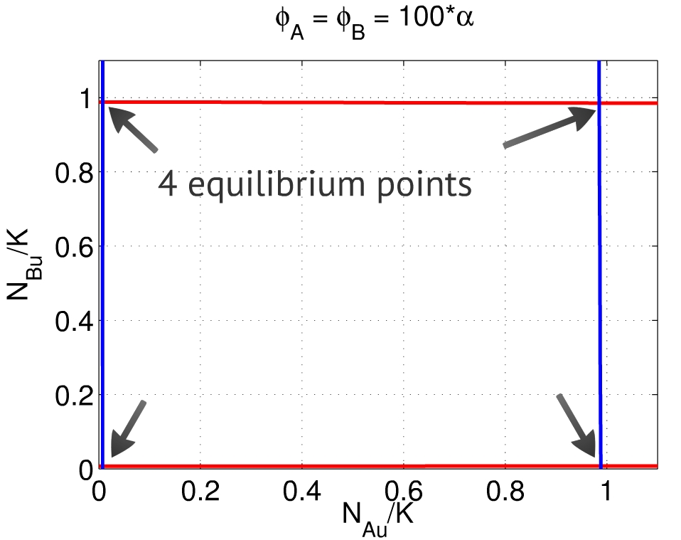
Finally, when both $\phi_A$ and $\phi_B$ are big when compared to $\alpha_A$ and $\alpha_B$, both populations A and B are able to
repress each other, depending on the initial conditions: there are equilibria both close to $(1,0)$ and to $(0,1)$ - with repression
of one population and activation of the other, Fig. 4.
Discussion
References
[1] J. P. Ward, J.R. King, A. J. Koerber, P. Williams, J. M. Croft and R. E. Sockett Mathematical modelling of quorum sensing in bacteria.
Math Med Biol (2001) 18(3)
[2] http://partsregistry.org/
 "
"


