Scaffold or Non-scaffold
Introduction
As explained before, the RNA scaffold brings the two enzymes (MS2 and PP7) closer, which improve the reaction rate of pathways. It seems magical that the reaction rate would be improved when two enzymes are close to each other. Then some questions are emerging. How faster it would be when two enzymes are in a RNA scaffold? What are the factors that will affect the efficiency of pathways? Those are what we want to discuss below. In this section, we establish a model by simplifying the molecular motion and simulating the reaction using Matlab programming.
Simplification
We simplify our abstract model as a pathway A -> B -> C. Enzyme one (E1) catalyzes the reaction A -> B and enzyme two (E2) catalyzes the reaction B -> C. The reaction equation is:
`A \leftrightarrow B \leftrightarrow C`
Molecular motion is continuous and complex so that it is difficult to model precisely. As a simplification, it is reasonable to discretize the continuous time as discrete steps and simplify the molecular Brownian motion as three-dimensional random walking. With this simplification, we can approximately observe the process of reaction and the reaction rate. Therefore, we present algorithms to simulate the process of molecular reaction dynamically and intuitionally.
Algorithm
In order to simulate the molecular motion and verify the fact that a RNA scaffold with two enzymes can speed reactions of the pathway, we simplify the complex realistic situation as a simple and virtual three dimensional world.
Assumptions:
1. The container is a cube and we assumed a unit. The edge of the cube is an integral multiple of one unit.
2. The cube is in a grid pattern and all the molecules are at the grid intersections.
3. The molecular motion is random walking in three dimensions.
4. The molecule cannot cross the edge of the cube.
Algorithm:
Initial state: All the molecules including A, E1 and E2 are randomly scattered at the intersections
Step 1: Check if there is A and E1 at the same intersection. If there, B is generated and A disappears.
Step 2: Check if there is B and E2 at the same intersection. If there, C is generated and B disappears.
Step 3: All the molecules are randomly walking one unit. If the molecule is going to across the border, it will be still and does not have a walk. Then, go back to step 1.
Implementation
We use the Matlab programming to construct the model and implement this algorithm, presenting the results using both data and 3D figures.
A small scale simulation
A small scale simulation is used to verify our algorithm, providing a clearly recognize of our algorithm.
The initial parameters are as followings:
Edge of cube: 30 units
The number of A: 200
The number of B: 0
The number of C: 0
The number of E1: 25
The number of E2: 25
The distance between E1 and E2 for RNA scaffold: 2 units
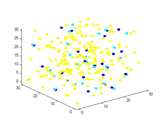
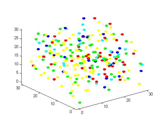
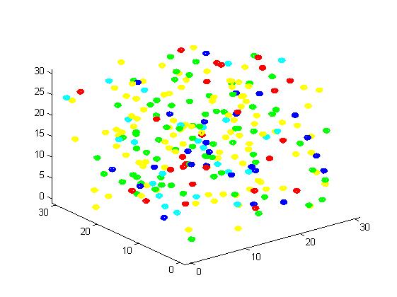
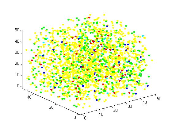
In the figure, we use the color yellow to represent A, green to B, red to C, blue to E1 and cyan to E2. This rule is used for all the figures in this section. The figures present the results vividly and visually. In addition, this is a random simulation so that we run the same code for 20 times and have an average outcome which is more convincing.
Figure 1. The initial state of the molecules for small scale simulation. The edge of cube is 30. There are 100 A, 25 E1 and 25 E2, which are randomly scattered in the cube container.
After 1000 iterations, the scaffold and non-scaffold results are as following:
Scaffold Non-scaffold
The number of A: 94 The number of A: 101
The number of B: 63 The number of B: 73
The number of C: 43 The number of C: 26
The number of E1: 25 The number of E1: 25
The number of E2: 25 The number of E2: 25
Figure 2. Result of scaffold system for small scale simulation. After 1000 iterations, there are 63 B and 43 C.
Figure 3. Result of non-scaffold system for small scale simulation. After 1000 iterations, there are 73 B and 26 C.
From the results, we can find that the number of C for scaffold is more than those for non-scaffold. Therefore, enzyme one and enzyme two being on a RNA scaffold can help to improve the reaction rate. The figures can help to provide a visible reflection. Though the small scale simulation has verified our algorithm, we also present a large scale simulation and have some discussion.
A large scale simulation
The initial state is as following:
Edge of cube: 50 units
The number of A: 2000
The number of B: 0
The number of C: 0
The number of E1: 50
The number of E2: 50
The distance between E1 and E2 for RNA scaffold: 2 units
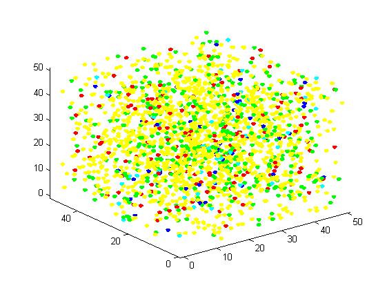
After 1200 iterations, the scaffold and non-scaffold results are as following:
Scaffold Non-scaffold
The number of A: 1417 The number of A: 1470
The number of B: 436 The number of B: 451
The number of C: 147 The number of C: 79
The number of E1: 50 The number of E1: 50
The number of E2: 50 The number of E2: 50
Figure 4. Result of scaffold system for large scale simulation. After 1200 iterations, there are 436 B and 147 C.
Figure 5. Result of non-scaffold system for large scale simulation. After 1200 iterations, there are 451 B and 79 C.
Comparison between scaffold system and non-scaffold system
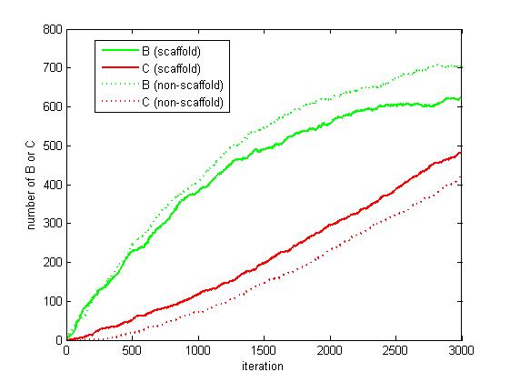
As the iteration increasing, the number of A is decreasing and the number of B and C are increasing. We record the number of B and C for both scaffold system and non-scaffold system as iteration grows to watch the reaction rate of pathway (i.e. the number of C).
Figure 6. The number of B and C as iteration grows.
From figure 4.5.6, it is obvious that the number of C for scaffold system is more than that for non-scaffold system and the number of B for scaffold system is less than that for non-scaffold system. This phenomenon can be interpreted as that the probability that B meets an E2 is highly increased since their distance is closer. Therefore, it is safely to draw a conclusion that the reaction rate of pathway has been speed up because of the scaffold bringing two enzymes closer.
Effect of enzymes concentration
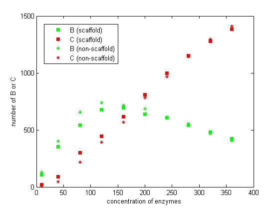
From the above discussion, we assumed the concentration of enzymes is constant. However, the increasing concentration of enzymes also results in the increasing of reaction rate. The difference between scaffold and non-scaffold system varies when the concentration of enzymes increase.
We select the number of E1 and E2 for 10, 40, 80, 120, 160, 200, 240, 280, 320 and 360 to record the number of C after 1200 iterations.
Figure 7. The number of B and C vary according to the concentration of enzymes.
From the figure 7, we find that when the concentration of enzymes is too low and too high, the difference between scaffold and non-scaffold system is not noticeable. Only when the concentration of enzymes is at a certain range of value, the advantages of scaffold system is significant. It seems reasonable that when the concentration is too low, the reaction rate is also low. When the concentration is too high, the probability that B meets an E2 is approximately equal for both systems.
Effect of distance between two enzymes
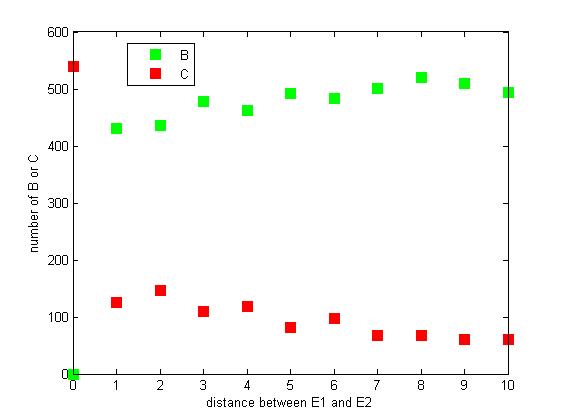
The distance between two enzymes E1 and E2 on RNA scaffold has an influence on reaction rate of pathway. If the E1 and E2 are closer, the probability that B, that is generated from A, meets an E2 is high for the reason that the distance between B and E2 are close. When the distance between E1 and E2 are getting further, the number of C is declining.
Figure 8. The number of B or C vary according to the distance between E1 and E2
From figure 8, it is easily to figure out that as the distance between E1 and E2 increasing, the final number of C is decreasing.
Binding analysis
Introduction
The binding of a RNA aptamer to MS2 or PP7 is dynamic, which means some MS2 and PP7 are binding with RNA aptamers and others are separated from RNA aptamers. Having known the initial concentration of RNA aptamer, MS2 and PP7, we need to find out how many RNA scaffolds have both MS2 and PP7 when the binding reach a final equilibrium. In this section, we use the concept -- association rate and dissociation rate [1] to model the process of binding.
Assumption
There are two aptamers on the RNA scaffold named aptamer1 (A1) and aptamer2 (A2). Aptamer1 is binding with MS2 and aptamer2 is binding with PP7. Before establishing the model, we declare some assumptions.
1.After mixing the RNA scaffold, MS2 and PP7, no RNA, MS2 and PP7 are added to the solution or removed from the solution.
2.MS2 would not bind with aptamer2 and PP7 would not bind with aptamer1.
3.The binding of MS2 to aptamer1 and the binding of PP7 to aptamer2 are independent with each other. The binding of one would not affect the binding of the other.
Symbols and Parameters Declaration
[`MS2`] : Concentration of MS2
[`PP7`] : Concentration of PP7
[`RNA`] : Concentration of RNA
[`A1`] : Concentration of aptamer1
[`A2`] : Concentration of aptamer2
[`MS2_0`] : The initial concentration of MS2
[`PP7_0`] : The initial concentration of PP7
[`RNA_0`] : The initial concentration of RNA
[`MS2A1`] : Concentration of MS2-Apatemer1(RNA) complex
[`MS2A1_0`] : The initial concentration of MS2-Apatemer1(RNA) complex
[`PP7A2`] : Concentration of PP7-Apatemer2(RNA) complex
[`PP7A2_0`] : The initial concentration of PP7-Apatemer2(RNA) complex
[`K_{+1}`] : Association rate of aptamer1 to MS2
[`K_{-1}`] : Dissociation rate of aptamer1 to MS2
[`K_{+2}`] : Association rate of aptamer2 to PP7
[`K_{-2}`] : Dissociation rate of aptamer2 to PP7
Differential equation modeling
The binding of aptamer1 to MS2 and aptamer2 to PP7 can be presented as reaction formula:
`MS2+A1 \leftrightarrow MS2A1`
`PP7+A2 \leftrightarrow PP7A2`
where MS2A1 is the MS2-A1 complex and PP7A2 is the PP7-A2.
According to the definition of association rate and dissociation rate, we can obtain the differential equations:
`\frac{d[MS2A1]}{dt}=k_{+1}[MS2][A1]-k_{-1}[MS2A1]`
`\frac{d[PP7A2]}{dt}=k_{+2}[PP7][A2]-k_{-2}[PP7A2]`
And it is obvious that
`[MS2]=[MS2_0]-[MS2A1][A1]=[RNA_0]-[MS2A1]`
`[PP7]=[PP7_0]-[PP7A2][A2]=[RNA_0]-[PP7A2]`
Therefore, we have the final differential equation
`\frac{d[MS2A1]}{dt}=k_{+1}([MS2_0]-[MS2A1])([RNA_0]-[MS2A1])-k_{-1}[MS2A1]`
`\frac{d[PP7A2]}{dt}=k_{+2}([PP7_0]-[PP7A2])([RNA_0]-[PP7A2])-k_{-2}[PP7A2]`
The initial value for `[MS2A1]` and `[PP7A2]` is
`[MS2A1_0]=0`
`[PP7A2_0]=0`
Equilibrium analysis
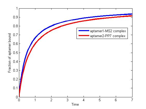
We solve the differential equations numerically using the "ode" solver in Matlab. Titolo et at once come up with an approach to determine the equilibrium dissociation constant. This constant is dependent on anisotropies of the sample, aptamer, and intensities of the polarizers[1]. Therefore, the association rate constant and dissociation rate constant are usually experimentally determined values. It is difficult for us to determine the constants precisely since they vary in terms of experimental environment.
According to literature, we assumed that
`k_{+1}=2 \times 10^4 M^{-1}S^{-1}`
`k_{-1}=2.18 \times 10^{-4} S^{-1}`
`k_{+2}=1.5 \times 10^4 M^{-1}S^{-1}`
`k_{-2}=1.63 \times 10^{-4} S^{-1}`
The results are shown as follows:
Figure 1. The fraction of aptamer1-MS2 complex and the fraction of aptamer2-PP7 complex are increasing and finally reach equilibrium.
As we mentioned above, the binding of MS2 to aptamer1 and the binding of PP7 to aptamer2 are independent with each other. The binding of one would not affect the binding of the other. From probability theoretical perspective, the fraction of RNA scaffold binding with both MS2 and PP7 is equal to the fraction of RNA scaffold binding with MS2 multiply the fraction of RNA scaffold binding with PP7. The RNA scaffold binding with both MS2 and PP7 is what we need to improve the reaction rate of pathways.
References
[1] Ajish S. R. Potty, Katerina Kourentzi, Han Fang, George W. Jackson, Xing Zhang, Glen B. Legge, Richard C. Willson. Biophysical Characterization of DNA Aptamer Interactions with Vascular Endothelial Growth Factor. 2008.

 "
"


