|
|
| (16 intermediate revisions not shown) |
| Line 92: |
Line 92: |
| | text-decoration: underline; | | text-decoration: underline; |
| | } | | } |
| | + | |
| | | | |
| | /* Bottom Environment (origin item) */ | | /* Bottom Environment (origin item) */ |
| Line 118: |
Line 119: |
| | { | | { |
| | font-family: Arial, sans-serif; | | font-family: Arial, sans-serif; |
| | + | font-size:16px; |
| | color: black; | | color: black; |
| | margin: 0; | | margin: 0; |
| | padding: 0; | | padding: 0; |
| | + | } |
| | + | |
| | + | /********************modified by MQ***************/ |
| | + | p.fig{ |
| | + | color: #573D01; |
| | + | padding: 15px 15px; |
| | + | font-size: 15.5px; |
| | + | font-family: "Calibri","sans-serif"; |
| | + | align: justify; |
| | + | } |
| | + | p.ref{ |
| | + | color: black; |
| | + | padding: 15px 15px; |
| | + | font-size: 15.5px; |
| | + | font-family: "Calibri","sans-serif"; |
| | + | align: justify; |
| | + | } |
| | + | b.orange{ |
| | + | color: #FF8000; |
| | + | font-style:italic; |
| | + | } |
| | + | .projectNav a { |
| | + | font-size: 18px; |
| | + | font-weight: bold; |
| | + | padding: 1px 5px; |
| | } | | } |
| | | | |
| Line 185: |
Line 212: |
| | | | |
| | #search-controls | | #search-controls |
| | + | { |
| | + | display: none; |
| | + | } |
| | + | |
| | + | #footer-box |
| | { | | { |
| | display: none; | | display: none; |
| Line 277: |
Line 309: |
| | | | |
| | <div id="main"> | | <div id="main"> |
| - | <h2 class="acc_trigger"><a href="http://thesum.ca/work.html#">01 <strong>Molecular Modeling</strong></a></h2> | + | <h2 class="acc_trigger">01 <strong>Molecular Modeling</strong></h2> |
| | <div class="acc_container" style="display: none; "> | | <div class="acc_container" style="display: none; "> |
| | <!--Content Goes Here--> | | <!--Content Goes Here--> |
| | | | |
| - | <p align="justify">In this year’s project, we try to make reasonable design of riboscaffolds by ourselves. Due to the current experimental conditions, we could not know what exactly happens to our riboscaffolds in the cell. Its folding process, binding with proteins and ligand, and the allosteric transition are of interests, since these are considerations for a reasonable design. Luckily, we have simulation tools for molecular modeling which can provide hints about what may happen theoretically in the intracellular environment. Although molecular modeling is often considered as professional work in which knowledge of different disciplines such as biology, physics, chemistry, mathematics and computer science as well as previous experience all contribute to good results, our team is willing to take a step in this field and get preliminary results.</p> | + | <div class="projectNav"> |
| - | <p align="justify"> </p>
| + | <p align="justify">In this year’s project, we try to make <b class="orange">reasonable design</b> of riboscaffolds by ourselves. Due to the current experimental conditions, we could not know what exactly happens to our riboscaffolds in the cell. Its folding process, binding with proteins and ligand, and the allosteric transition are of interests, since these are considerations for a reasonable design. Luckily, we have <b class="orange">simulation tools</b> for molecular modeling which can provide hints about <b class="orange">what may happen theoretically in the intracellular environment</b>. Although molecular modeling is often considered as professional work in which knowledge of different disciplines such as biology, physics, chemistry, mathematics and computer science as well as previous experience all contribute to good results, our team is willing to take a step in this field and get preliminary results.</p> |
| - | <h3>RNA folding and 3D Structures</h3>
| + | |
| - | <p align="justify"> </p>
| + | |
| - | <h5>Introduction</h5>
| + | |
| - | <p align="justify"> </p>
| + | |
| - | <p align="justify">For most small RNA molecules, secondary structure is enough for predicting their possible functions since their size limits their ability to fold into complex structures. However, our riboscaffold is a large one of 100~160 bp and has several arms. As in addition, our design of kissing loop is on the level of tertiary structure. So it is helpful if we can simulate RNA folding in silico.</p>
| + | |
| - | <p align="justify"> </p>
| + | |
| - | <h5>Methods</h5>
| + | |
| - | <p align="justify"> </p>
| + | |
| - | <p align="justify">NAST/C2A [10] is a set of Python tools that can generate full-atomic 3D RNA structures from secondary structure information. NAST generates coarse grained 3D structures from secondary structure information, and C2A adds the full-atomic details to these coarse-grained models. PyOpenMM [11] was required, VMD [12] and PyMOL [13] was used to view the results and trajectories.</p>
| + | |
| - | <p align="justify"> </p>
| + | |
| - | <p align="justify">Beginning with sequences and secondary structures, NAST generates 3D structures in two different ways. The first is to start an MD simulation from an unfolded circle state. The second is a more sophisticate approach that starts at a random position in the sequence, and adds residues to each end at a random plausible position. Details about the sequences and design strategy can be found here.</p>
| + | |
| - | <p align="justify"> </p>
| + | |
| - | <h5>Results</h5>
| + | |
| - | <p align="justify"> </p>
| + | |
| - | <p align="justify">The following two movies about the folding process of D0 explain the two different ways of 3D structure prediction provided by NAST. </p>
| + | |
| - | <p align="justify"> </p>
| + | |
| - | <p align="justify">Movie1. Start an MD simulation from an unfolded circle state.</p>
| + | |
| - | <p align="justify"> </p>
| + | |
| - | <p align="justify">Movie2. Starts at a random position in the sequence, and adds residues to each end at a random plausible position.</p>
| + | |
| - | <p align="justify"> </p>
| + | |
| - | <p align="justify">According to the document of NAST, the second method (random unfold starting structure) is more sophisticate, so in the following movies, we use this method to predict the folding of the riboscaffolds we designed.</p>
| + | |
| - | <p align="justify"> </p>
| + | |
| - | <p align="justify"><img src="https://static.igem.org/mediawiki/igem.org/2/24/Zju_model1_1.png" width="500px" /></p>
| + | |
| - | <p align="justify"> </p>
| + | |
| - | <p align="justify">Figure 1. Clover1 3D structure Movie3. Clover1 Folding.</p>
| + | |
| - | <p align="justify"> </p>
| + | |
| - | <p align="justify"><img src="https://static.igem.org/mediawiki/igem.org/d/d3/Zju_model1_2.png" width="500px" /></p>
| + | |
| - | <p align="justify"> </p>
| + | |
| - | <p align="justify">Figure 2 Colver2-1 structure Movie4. One possible folding process of Clover2. </p>
| + | |
| - | <p align="justify"> </p>
| + | |
| - | <p align="justify">In this conformation, the interaction between theophylline aptamer and MS2 aptamer is not obvious, probably because they extend from the same loop, which is too small to be flexible. </p>
| + | |
| - | <p align="justify"> </p>
| + | |
| - | <p align="justify"><img src="https://static.igem.org/mediawiki/igem.org/f/ff/Zju_model1_3.png" width="500px" /></p>
| + | |
| - | <p align="justify"> </p>
| + | |
| - | <p align="justify">Figure 3 Colver2-1 structure Movie5. Another possible folding process of Clover2. </p>
| + | |
| - | <p align="justify"> </p>
| + | |
| - | <p align="justify">In this conformation, the interaction between theophylline aptamer can be seen during the folding process, but as the MS2 aptamer extends, the internal rigidity pretends the torsion in the structure.</p>
| + | |
| - | <p align="justify"> </p>
| + | |
| - | <p align="justify"><img src="https://static.igem.org/mediawiki/igem.org/f/f9/Zju_model1_4.png" width="500px" /></p>
| + | |
| - | <p align="justify"> </p>
| + | |
| - | <p align="justify">Figure 4 Colver3 structure. Movie6. Clover3 folding. </p>
| + | |
| - | <p align="justify"> </p>
| + | |
| - | <p align="justify">In this movie, we can see the interaction between theophylline aptamer and MS2 aptamer is more obvious, which begins from the formation of MS2 and remains in the “mature” Clover3.</p>
| + | |
| - | <p align="justify"> </p>
| + | |
| - | <p align="justify"><img src="https://static.igem.org/mediawiki/igem.org/0/05/Zju_model1_5.png" width="500px" /></p>
| + | |
| - | <p align="justify"> </p>
| + | |
| - | <p align="justify">Figure 5 Clover3 mutant. Movie7. Clover3 mutant folding</p>
| + | |
| - | <p align="justify"> </p>
| + | |
| - | <p align="justify">To demonstrate that the interaction in Clover3 is caused by our design, we simulate the 3D structure of a mutant of Clover 3, in which the theophylline aptamer remains unmutant so it cannot base pair with the sequence of MS2.</p>
| + | |
| - | <p align="justify"> </p>
| + | |
| - | <h3>Docking</h3>
| + | |
| - | <p align="justify"> </p>
| + | |
| - | <h5>Introduction</h5>
| + | |
| - | <p align="justify"> </p>
| + | |
| - | <p align="justify">Docking is a method which predicts the preferred orientation and binding affinity of one molecule to a second when bound to each other to form a stable complex. Docking is frequently used to predict the binding orientation of small molecule drug candidates to their protein targets in order to in turn predict the affinity and activity of the small molecule. Hence docking plays an important role in the rational design of drugs.</p>
| + | |
| - | <p align="justify"> </p>
| + | |
| - | <p align="justify">In our cases, riboscaffolds are designed as targets of small ligands, so we can dock the ligand to the riboscaffold to find the binding site and evaluate the binding state. </p>
| + | |
| - | <p align="justify"> </p>
| + | |
| - | <h5>Methods</h5>
| + | |
| - | <p align="justify"> </p>
| + | |
| - | <p align="justify">Although most docking algorithms and tools, as well as tutorials and documents are designed for drug-protein docking, we managed to find several approaches to conduct docking on RNA aptamers[1,2], which is a heating ground in the research of RNA targeting drugs. Among the popular docking tools, AutoDock package [3] has demonstrated its ability to dock compounds to RNA molecules [1]. In our approach, we docked theophylline to our riboscaffolds (with the predicted 3D structure) to search for the binding sites and construct ligand-riboscaffold complex for dynamic analysis.</p>
| + | |
| - | <p align="justify"> </p>
| + | |
| - | <p align="justify">Step1: Preparation of riboscaffold</p>
| + | |
| - | <p align="justify"> </p>
| + | |
| - | <p align="justify">The coordinate files predicted by Nast, refined by C2A, balanced and optimized by OpenMM Zephyr were used for docking. But they can still have potential problems that need to be corrected. The preparation was done in AutoDock Tools, including merging the non-polar hydrogen atoms on RNA molecules and computing Gasteiger charges. Then, the PDB files were converted to PDBQT files used in AutoDock. </p>
| + | |
| - | <p align="justify"> </p>
| + | |
| - | <p align="justify">Step2: Preparation of theophylline.</p>
| + | |
| - | <p align="justify"> </p>
| + | |
| - | <p align="justify">The ligand theophylline was obtained from chEBI database (www.ebi.ac.uk/chebi/) as MOL file and converted to PDB coordinate file using OpenBable [4]. Preparation was performed also in AutoDock Tools, and because the molecule of theophylline is quite rigid, there is no need to specify rotatable bonds and active torsions, just used the default settings and generated PDBQT file.</p>
| + | |
| - | <p align="justify"> </p>
| + | |
| - | <p align="justify">Step3: Run docking with AutoDock.</p>
| + | |
| - | <p align="justify"> </p>
| + | |
| - | <p align="justify">Once the receptor and ligand are prepared, we can use the AutoDock 4.2 package. The grid box for site searching was created on different arms on our riboscaffolds according to their dimensions with the default 0.375 angstrom for spacing between the grid points. For each riboscaffold, 20 docking experiments were performed using the Lamarckian genetic algorithm conformational search, with the population size of 150, one million energy evaluations, and a maximum of 27 000 generations per run.</p>
| + | |
| - | <p align="justify"> </p>
| + | |
| - | <h5>Results</h5>
| + | |
| - | <p align="justify"> </p>
| + | |
| - | <p align="justify"><img src="https://static.igem.org/mediawiki/igem.org/e/ee/Zju_model1_6.png" width="500px" /></p>
| + | |
| - | <p align="justify"> </p>
| + | |
| - | <p align="justify">Figure6. This figure shows the docking result of the three arms (theophylline aptamer, MS2 aptamer and PP7 aptamer). Ligands are in white.</p>
| + | |
| - | <p align="justify"> </p>
| + | |
| - | <p align="justify">There are more binding sites of theophylline on the theophylline aptamer than on the other two aptamers, which indicates the present of theophylline is highly probable to have some effects on the theophylline aptamer. And the effects caused by theophylline is mainly through its interation with theophylline aptamer, which is consistent with our experimental results. </p>
| + | |
| - | <p align="justify"> </p>
| + | |
| - | <p align="justify">The docking results were used to generate riboscaffold-theophylline complex for molecular dynamics analysis of the whole system.</p>
| + | |
| - | <p align="justify"> </p>
| + | |
| - | <h3>Molecular Dynamics</h3>
| + | |
| - | <p align="justify"> </p>
| + | |
| - | <h5>Introduction</h5>
| + | |
| - | <p align="justify"> </p>
| + | |
| - | <p align="justify">Molecular dynamics (MD) is a computer simulation of physical movements of atoms and molecules. The atoms and molecules are allowed to interact for a period of time, giving a view of the motion of the atoms by numerically solving the Newton's equations. The results of molecular dynamics simulations includes the trajectory of molecules and atoms in the system and other parameters such as energy potential, temperature and pressure fluctuations, number of hydrogen bonds of the system, which may be used to find the properties of such complex systems analytically. </p>
| + | |
| - | <p align="justify"> </p>
| + | |
| - | <h5>Methods</h5>
| + | |
| - | <p align="justify"> </p>
| + | |
| - | <p align="justify">Here in our project, we use GROMACS 4.5 [5] to run MD and analyze the state of theophylline-riboscaffold complex. GROMACS is a versatile package to perform molecular dynamics on macromolecules like proteins, lipids and nucleic acids. It is fast, has multiple choices for force field, and comes with a large selection of flexible tools for trajectory analysis. </p>
| + | |
| - | <p align="justify"> </p>
| + | |
| - | <p align="justify">Although GROMACS provides step by step tutorials for beginners, they are all for proteins or protein-ligand complex. Our riboscaffold-theophylline system is similar to protein-ligand complex to some degree, but they have their own characteristics. We, as beginners, are trying to develop a protocol for the MD simulation of ligand sensible RNA devices based on canonical tutorials for protein-ligand complex [6, 7]. It may be coarse now, and we will modify it and add more details after more experiments, we hope it is helpful for people who are also beginners and interested in RNA molecular dynamics.</p>
| + | |
| - | <p align="justify"> </p>
| + | |
| - | <p align="justify">Step1: Separate the RNA and ligand from a complex file.</p>
| + | |
| - | <p align="justify">We used the complex file generated by AutoDock and separate them into two PDB files with the coordinate of atoms conserved. </p>
| + | |
| - | <p align="justify"> </p>
| + | |
| - | <p align="justify">Step2: Prepare the protein topology with pdb2gmx.</p>
| + | |
| - | <p align="justify">Choose AMBER force fields because they are more suitable for RNA MD. In our cases, we chose AMBER99SB.</p>
| + | |
| - | <p align="justify"> </p>
| + | |
| - | <p align="justify">Step3: Prepare the ligand topology using external tools.</p>
| + | |
| - | <p align="justify">Proper treatment of ligands is one of the most challenging tasks in molecular simulation. The ligand should be treated with the force field that is consistent with the receptor. Unlike the tutorials for protein-ligand complex, in which the PRODRG web server with GROMOS force field is used, we prepared our ligand with Antechamber [8] and tleap [9], free tools in the AmberTools package. The output files are a top and a gro file for the ligand. The top file should be converted into itp file for reusability and included in the receptor top file.</p>
| + | |
| - | <p align="justify"> </p>
| + | |
| - | <p align="justify">Step4: Solvation</p>
| + | |
| - | <p align="justify">At this point, it is necessary to define the unit cell and fill it with water, just as described in other tutorials for any other MD simulation.</p>
| + | |
| - | <p align="justify"> </p>
| + | |
| - | <p align="justify">Step5: Adding ions</p>
| + | |
| - | <p align="justify">A .tpr file must be generated for the input. Therefore, we will setup energy minimization, which means running grompp before genion. Energy minimization in this step is different form that in the following step, here we just want to know the charges of our system. Our system has a net charge of -157e, so we add 157 Na+ to simulate the status in cytoplasm. </p>
| + | |
| - | <p align="justify"> </p>
| + | |
| - | <p align="justify">Step6: Energy Minimization</p>
| + | |
| - | <p align="justify">Having added ions, we need to rerun energy minimization. In the .mdp file, remember to set energygrps to the right names of the elements in the system. It is recommended to checked the [molecule] part of the .top file to make sure all kinds of molecules in the system are correctly included.</p>
| + | |
| - | <p align="justify"> </p>
| + | |
| - | <p align="justify">Step7: Equilibration</p>
| + | |
| - | <p align="justify">Similar to the protein-ligand complex, in the stage of equilibration, we should first restrain our ligand (but it is not fixed!) around the binding site during equilibration, control the temperature coupling, and run two phases of equilibration, NVT (canonical ensemble, moles N, volume V and temperature T are conserved.) and NPT (isothermal–isobaric ensemble, in which moles N, pressure P and temperature T are conserved.)</p>
| + | |
| - | <p align="justify"> </p>
| + | |
| - | <p align="justify">Step8: Production MD</p>
| + | |
| - | <p align="justify">After two phases of equilibration, the system has reached the desired temperature and pressure. So we will run MD again and get the products.</p>
| + | |
| - | <p align="justify"> </p>
| + | |
| - | <h5>Results</h5>
| + | |
| - | <p align="justify"> </p>
| + | |
| - | <p align="justify"><img src="https://static.igem.org/mediawiki/igem.org/c/cd/Zju_model1_7.png" width="500px" /></p>
| + | |
| - | <p align="justify"> </p>
| + | |
| - | <p align="justify">Figure 7. The potential energy of the system.</p>
| + | |
| - | <p align="justify"> </p>
| + | |
| - | <p align="justify">The potential energy equilibrates about an average of ~ –3274000 kJ/mol.</p>
| + | |
| - | <p align="justify"> </p>
| + | |
| - | <p align="justify"><img src="https://static.igem.org/mediawiki/igem.org/4/4c/Zju_model1_8.png" width="500px" /></p>
| + | |
| - | <p align="justify"> </p>
| + | |
| - | <p align="justify">Figure 8. Temperature fluctuation.</p>
| + | |
| - | <p align="justify"> </p>
| + | |
| - | <p align="justify"><img src="https://static.igem.org/mediawiki/igem.org/f/fe/Zju_model1_9.png" width="500px" /></p>
| + | |
| - | <p align="justify"> </p>
| + | |
| - | <p align="justify">Figure 9. Pressure fluctuation.</p>
| + | |
| - | <p align="justify"> </p>
| + | |
| - | <p align="justify">The temperature and pressure plot shows the normal oscillation behavior. The average temperature is about 310 K, which is what we desired.</p>
| + | |
| - | <p align="justify"> </p>
| + | |
| - | <p align="justify"><img src="https://static.igem.org/mediawiki/igem.org/3/3e/Zju_model1_10.png" width="500px" /></p>
| + | |
| - | <p align="justify"> </p>
| + | |
| - | <p align="justify">Figure 10. Hydrogen bonds.</p>
| + | |
| - | <p align="justify"> </p>
| + | |
| - | <p align="justify">The number of hydrogen bonds ranges mainly between 3 and 4. This figure shows the interaction is rather stable.</p>
| + | |
| - | <p align="justify"> </p>
| + | |
| - | <p align="justify"><img src="https://static.igem.org/mediawiki/igem.org/8/8b/Zju_model1_11.png" width="500px" /></p>
| + | |
| - | <p align="justify"> </p>
| + | |
| - | <p align="justify">Figure 11. RMSD of RNA.</p>
| + | |
| - | <p align="justify"> </p>
| + | |
| - | <p align="justify"><img src="https://static.igem.org/mediawiki/igem.org/4/40/Zju_model1_12.png" width="500px" /></p>
| + | |
| - | <p align="justify"> </p>
| + | |
| - | <p align="justify">Figure 12. RMSD of theophylline.</p>
| + | |
| - | <p align="justify"> </p>
| + | |
| - | <p align="justify">The two figures about RMSD indicates that the RNA, as a receptor, equilibrates rather quickly. But the small ligand, theophylline, equilibrates slower, with a larger range of fluctuation (about 0.02, but in RNA, the range is within 0.05) in conformation. This is normal in ligand-receptor systems. </p>
| + | |
| - | <p align="justify"> </p>
| + | |
| - | <p align="justify">In conclusion, the preliminary analysis results show that the simulation system generated by our workflow acts similar to other ligand-receptor systems under the environment of molecular dynamics. Actually, with this method, we can conduct more analysis on the level of molecules and even atoms. We will continue our way to explore this magic microworld!</p>
| + | |
| - | <p align="justify"> </p>
| + | |
| - | <h3>References</h3>
| + | |
| - | <p align="justify"> </p>
| + | |
| - | <p align="justify">[1] Yaroslav Chushak, Morley O. Stone. In silico selection of RNA aptamers. Nucl. Acids Res. (2009) 37(12).( http://nar.oxfordjournals.org/content/37/12/e87.short)</p>
| + | |
| - | <p align="justify"> </p>
| + | |
| - | <p align="justify">[2] Florent Barbault. RNA as drug target: docking studies. </p>
| + | |
| - | <p align="justify"> </p>
| + | |
| - | <p align="justify">[3] Morris, G. M., Huey, R., Lindstrom, W., Sanner, M. F., Belew, R. K., Goodsell, D. S. and Olson, A. J. (2009) Autodock4 and AutoDockTools4: automated docking with selective receptor flexiblity. J. Computational Chemistry, 16: 2785-91.</p>
| + | |
| - | <p align="justify"> </p>
| + | |
| - | <p align="justify">[4] N M O'Boyle, M Banck, C A James, C Morley, T Vandermeersch, and G R Hutchison. "Open Babel: An open chemical toolbox." J. Cheminf. (2011), 3, 33.</p>
| + | |
| - | <p align="justify"> </p>
| + | |
| - | <p align="justify">[5] Hess, et al. (2008) GROMACS 4: Algorithms for Highly Efficient, Load-Balanced, and Scalable Molecular Simulation. J. Chem. Theory Comput. 4: 435-447.</p>
| + | |
| - | <p align="justify"> </p>
| + | |
| - | <p align="justify">[6] John E. Kerrigan. GROMACS Tutorial for Drug – Enzyme Complex.</p>
| + | |
| - | <p align="justify"> </p>
| + | |
| - | <p align="justify">[7] Justin Lemkul. GROMACS Tutorial: Protein-Ligand Complex. (http://www.bevanlab.biochem.vt.edu/Pages/Personal/justin/gmx-tutorials/complex/index.html)</p>
| + | |
| - | <p align="justify"> </p>
| + | |
| - | <p align="justify">[8] Wang, J., Wang, W., Kollman P. A.; Case, D. A. "Automatic atom type and bond type perception in molecular mechanical calculations". Journal of Molecular Graphics and Modelling , 25, 2006, 247260.</p>
| + | |
| - | <p align="justify"> </p>
| + | |
| - | <p align="justify">[9] Christian E. A. F. Schafmeister, Wilson S. Ross and Vladimir Romanovski, , University of California, San Francisco (1995).</p>
| + | |
| - | <p align="justify"> </p>
| + | |
| - | <p align="justify">[10] Jonikas MA, Radmer RJ, Laederach A, Das R, Pearlman S, Herschlag D, Altman RB. Coarse-grained modeling of large RNA molecules with knowledge-based potentials and structural filters. RNA. 2009 Feb;15(2):189-99. PMID: 19144906 (2009).</p>
| + | |
| - | <p align="justify"> </p>
| + | |
| - | <p align="justify">[11] M. S. Friedrichs, P. Eastman, V. Vaidyanathan, M. Houston, S. LeGrand, A. L. Beberg, D. L. Ensign, C. M. Bruns, V. S. Pande. “Accelerating Molecular Dynamic Simulation on Graphics Processing Units.” J. Comp. Chem., 30(6), 864-872. (2009) (https://simtk.org/home/pyopenmm)</p>
| + | |
| - | <p align="justify"> </p>
| + | |
| - | <p align="justify">[12] Humphrey, W., Dalke, A. and Schulten, K., "VMD - Visual Molecular Dynamics", J. Molec. Graphics, 1996, vol. 14, pp. 33-38. (http://www.ks.uiuc.edu/Research/vmd/)</p>
| + | |
| - | <p align="justify"> </p>
| + | |
| - | <p align="justify">[13] The PyMOL Molecular Graphics System, Version 1.5.0.4 Schr?dinger, LLC.</p>
| + | |
| | <p align="justify"> </p> | | <p align="justify"> </p> |
| | + | |
| | + | <div class="projectNavFloat"> |
| | + | <a target="brainFrame" href="https://2012.igem.org/Team:ZJU-China/model_s1_1.htm" style="text-decoration:none">1. RNA folding and 3D Structures</a> |
| | + | <br> |
| | + | <a target="brainFrame" href="https://2012.igem.org/Team:ZJU-China/model_s1_2.htm" style="text-decoration:none">2. Docking</a> |
| | + | </div><!-- end .projectNavFloat --> |
| | + | <div class="projectNavFloat"> |
| | + | <a target="brainFrame" href="https://2012.igem.org/Team:ZJU-China/model_s1_3.htm" style="text-decoration:none">3. Molecular Dynamics</a> |
| | + | <br> |
| | + | <a target="brainFrame" href="https://2012.igem.org/Team:ZJU-China/model_s1_4.htm" style="text-decoration:none">4. References</a> |
| | + | |
| | + | </div><!-- end .projectNavFloat --> |
| | + | <br class="clearfloat"> |
| | + | </div><!-- end .projectNav --> |
| | + | |
| | + | <iframe src="" frameborder="0" name="brainFrame" width="100%" height="500px"> </iframe> |
| | | | |
| | | | |
| | </div><!-- end .acc_container --> | | </div><!-- end .acc_container --> |
| | | | |
| - | <h2 class="acc_trigger"><a href="http://thesum.ca/work.html#">02 <strong>Scaffold or Non-scaffold</strong></a></h2> | + | <h2 class="acc_trigger">02 <strong>Scaffold or Non-scaffold</strong></h2> |
| | <div class="acc_container" style="display: none; "> | | <div class="acc_container" style="display: none; "> |
| | <!--Content Goes Here--> | | <!--Content Goes Here--> |
| - | <h3>Introduction</h3> | + | <div class="projectNav"> |
| - | <p align="justify"> </p>
| + | |
| | <p align="justify">As explained before, the RNA scaffold brings the two enzymes (MS2 and PP7) closer, which improve the reaction rate of pathways. It seems magical that the reaction rate would be improved when two enzymes are close to each other. Then some questions are emerging. How faster it would be when two enzymes are in a RNA scaffold? What are the factors that will affect the efficiency of pathways? Those are what we want to discuss below. In this section, we establish a model by simplifying the molecular motion and simulating the reaction using Matlab programming.</p> | | <p align="justify">As explained before, the RNA scaffold brings the two enzymes (MS2 and PP7) closer, which improve the reaction rate of pathways. It seems magical that the reaction rate would be improved when two enzymes are close to each other. Then some questions are emerging. How faster it would be when two enzymes are in a RNA scaffold? What are the factors that will affect the efficiency of pathways? Those are what we want to discuss below. In this section, we establish a model by simplifying the molecular motion and simulating the reaction using Matlab programming.</p> |
| | <p align="justify"> </p> | | <p align="justify"> </p> |
| - | <h3>Simplification</h3>
| |
| - | <p align="justify"> </p>
| |
| - | <p align="justify">We simplify our abstract model as a pathway A -> B -> C. Enzyme one (E1) catalyzes the reaction A -> B and enzyme two (E2) catalyzes the reaction B -> C. The reaction equation is:</p>
| |
| - | <p align="justify"> </p>
| |
| - | <p align="justify">`A \leftrightarrow B \leftrightarrow C`</p>
| |
| - | <p align="justify"> </p>
| |
| - | <p align="justify">Molecular motion is continuous and complex so that it is difficult to model precisely. As a simplification, it is reasonable to discretize the continuous time as discrete steps and simplify the molecular Brownian motion as three-dimensional random walking. With this simplification, we can approximately observe the process of reaction and the reaction rate. Therefore, we present algorithms to simulate the process of molecular reaction dynamically and intuitionally.</p>
| |
| - | <p align="justify"> </p>
| |
| - | <h3>Algorithm</h3>
| |
| - | <p align="justify"> </p>
| |
| - | <p align="justify">In order to simulate the molecular motion and verify the fact that a RNA scaffold with two enzymes can speed reactions of the pathway, we simplify the complex realistic situation as a simple and virtual three dimensional world.</p>
| |
| - | <p align="justify"> </p>
| |
| - | <h3>Assumptions:</h3>
| |
| - | <p align="justify"> </p>
| |
| - | <p align="justify">1. The container is a cube and we assumed a unit. The edge of the cube is an integral multiple of one unit.</p>
| |
| - | <p align="justify"> </p>
| |
| - | <p align="justify">2. The cube is in a grid pattern and all the molecules are at the grid intersections.</p>
| |
| - | <p align="justify"> </p>
| |
| - | <p align="justify">3. The molecular motion is random walking in three dimensions.</p>
| |
| - | <p align="justify"> </p>
| |
| - | <p align="justify">4. The molecule cannot cross the edge of the cube.</p>
| |
| - | <p align="justify"> </p>
| |
| - | <h3>Algorithm:</h3>
| |
| - | <p align="justify"> </p>
| |
| - | <p align="justify">Initial state: All the molecules including A, E1 and E2 are randomly scattered at the intersections</p>
| |
| - | <p align="justify"> </p>
| |
| - | <p align="justify">Step 1: Check if there is A and E1 at the same intersection. If there, B is generated and A disappears.</p>
| |
| - | <p align="justify"> </p>
| |
| - | <p align="justify">Step 2: Check if there is B and E2 at the same intersection. If there, C is generated and B disappears.</p>
| |
| - | <p align="justify"> </p>
| |
| - | <p align="justify">Step 3: All the molecules are randomly walking one unit. If the molecule is going to across the border, it will be still and does not have a walk. Then, go back to step 1.</p>
| |
| - | <p align="justify"> </p>
| |
| - | <h3>Implementation</h3>
| |
| - | <p align="justify"> </p>
| |
| - | <p align="justify">We use the Matlab programming to construct the model and implement this algorithm, presenting the results using both data and 3D figures.</p>
| |
| - | <p align="justify"> </p>
| |
| - | <h3>A small scale simulation</h3>
| |
| - | <p align="justify"> </p>
| |
| - | <p align="justify">A small scale simulation is used to verify our algorithm, providing a clearly recognize of our algorithm. </p>
| |
| - | <p align="justify"> </p>
| |
| - | <p align="justify">The initial parameters are as followings:</p>
| |
| - | <p align="justify">Edge of cube: 30 units</p>
| |
| - | <p align="justify">The number of A: 200</p>
| |
| - | <p align="justify">The number of B: 0</p>
| |
| - | <p align="justify">The number of C: 0</p>
| |
| - | <p align="justify">The number of E1: 25</p>
| |
| - | <p align="justify">The number of E2: 25</p>
| |
| - | <p align="justify">The distance between E1 and E2 for RNA scaffold: 2 units</p>
| |
| - | <p align="justify"> </p>
| |
| - | <p align="justify">In the figure, we use the color yellow to represent A, green to B, red to C, blue to E1 and cyan to E2. This rule is used for all the figures in this section. The figures present the results vividly and visually. In addition, this is a random simulation so that we run the same code for 20 times and have an average outcome which is more convincing.</p>
| |
| - | <div><img src="http://www.jiajunlu.com/igem/zju_model2_1.jpg"></div>
| |
| | | | |
| - | <p align="justify">Figure 1. The initial state of the molecules for small scale simulation. The edge of cube is 30. There are 100 A, 25 E1 and 25 E2, which are randomly scattered in the cube container.
| |
| - | After 1000 iterations, the scaffold and non-scaffold results are as following:</p>
| |
| - | <p align="justify"> </p>
| |
| - | <p align="justify">Scaffold Non-scaffold</p>
| |
| - | <p align="justify">The number of A: 94 The number of A: 101</p>
| |
| - | <p align="justify">The number of B: 63 The number of B: 73</p>
| |
| - | <p align="justify">The number of C: 43 The number of C: 26</p>
| |
| - | <p align="justify">The number of E1: 25 The number of E1: 25</p>
| |
| - | <p align="justify">The number of E2: 25 The number of E2: 25</p>
| |
| - | <p align="justify"> </p>
| |
| - | <div><img src="http://www.jiajunlu.com/igem/zju_model2_2.jpg"></div>
| |
| - | <p align="justify">Figure 2. Result of scaffold system for small scale simulation. After 1000 iterations, there are 63 B and 43 C.</p>
| |
| - | <div><img src="http://www.jiajunlu.com/igem/zju_model2_3.jpg"></div>
| |
| - | <p align="justify">Figure 3. Result of non-scaffold system for small scale simulation. After 1000 iterations, there are 73 B and 26 C.</p>
| |
| - | <p align="justify"> </p>
| |
| - | <p align="justify">From the results, we can find that the number of C for scaffold is more than those for non-scaffold. Therefore, enzyme one and enzyme two being on a RNA scaffold can help to improve the reaction rate. The figures can help to provide a visible reflection. Though the small scale simulation has verified our algorithm, we also present a large scale simulation and have some discussion.</p>
| |
| - | <p align="justify"> </p>
| |
| - | <h3>A large scale simulation</h3>
| |
| - | <p align="justify">The initial state is as following:</p>
| |
| - | <p align="justify">Edge of cube: 50 units</p>
| |
| - | <p align="justify">The number of A: 2000</p>
| |
| - | <p align="justify">The number of B: 0</p>
| |
| - | <p align="justify">The number of C: 0</p>
| |
| - | <p align="justify">The number of E1: 50</p>
| |
| - | <p align="justify">The number of E2: 50</p>
| |
| - | <p align="justify">The distance between E1 and E2 for RNA scaffold: 2 units</p>
| |
| - | <p align="justify"> </p>
| |
| - | <p align="justify">After 1200 iterations, the scaffold and non-scaffold results are as following:</p>
| |
| - | <p align="justify">Scaffold Non-scaffold</p>
| |
| - | <p align="justify">The number of A: 1417 The number of A: 1470</p>
| |
| - | <p align="justify">The number of B: 436 The number of B: 451</p>
| |
| - | <p align="justify">The number of C: 147 The number of C: 79</p>
| |
| - | <p align="justify">The number of E1: 50 The number of E1: 50</p>
| |
| - | <p align="justify">The number of E2: 50 The number of E2: 50</p>
| |
| - | <div><img src="http://www.jiajunlu.com/igem/zju_model2_4.jpg"></div>
| |
| - | <p align="justify">Figure 4. Result of scaffold system for large scale simulation. After 1200 iterations, there are 436 B and 147 C.</p>
| |
| - | <div><img src="http://www.jiajunlu.com/igem/zju_model2_5.jpg"></div>
| |
| - | <p align="justify">Figure 5. Result of non-scaffold system for large scale simulation. After 1200 iterations, there are 451 B and 79 C.</p>
| |
| - | <p align="justify"> </p>
| |
| - | <h3>Comparison between scaffold system and non-scaffold system</h3>
| |
| - | <p align="justify">As the iteration increasing, the number of A is decreasing and the number of B and C are increasing. We record the number of B and C for both scaffold system and non-scaffold system as iteration grows to watch the reaction rate of pathway (i.e. the number of C).</p>
| |
| - | <div><img src="http://www.jiajunlu.com/igem/zju_model2_6.jpg"></div>
| |
| - | <p align="justify">Figure 6. The number of B and C as iteration grows.</p>
| |
| - | <p align="justify"> </p>
| |
| - | <p align="justify">From figure 4.5.6, it is obvious that the number of C for scaffold system is more than that for non-scaffold system and the number of B for scaffold system is less than that for non-scaffold system. This phenomenon can be interpreted as that the probability that B meets an E2 is highly increased since their distance is closer. Therefore, it is safely to draw a conclusion that the reaction rate of pathway has been speed up because of the scaffold bringing two enzymes closer.</p>
| |
| | | | |
| - | <h3>Effect of enzymes concentration</h3> | + | <div class="projectNavFloat"> |
| - | <p align="justify">From the above discussion, we assumed the concentration of enzymes is constant. However, the increasing concentration of enzymes also results in the increasing of reaction rate. The difference between scaffold and non-scaffold system varies when the concentration of enzymes increase.</p> | + | <a target="brainFramei" href="https://2012.igem.org/Team:ZJU-China/model_s2_1.htm" style="text-decoration:none">1. Preparation</a> |
| - | <p align="justify"> </p>
| + | <br> |
| - | <p align="justify">We select the number of E1 and E2 for 10, 40, 80, 120, 160, 200, 240, 280, 320 and 360 to record the number of C after 1200 iterations.</p> | + | <a target="brainFramei" href="https://2012.igem.org/Team:ZJU-China/model_s2_2.htm" style="text-decoration:none">2. A small scale simulation</a> |
| - | <div><img src="http://www.jiajunlu.com/igem/zju_model2_7.jpg"></div> | + | </div><!-- end .projectNavFloat --> |
| - | <p align="justify">Figure 7. The number of B and C vary according to the concentration of enzymes.</p> | + | <div class="projectNavFloat"> |
| - | <p align="justify"> </p> | + | <a target="brainFramei" href="https://2012.igem.org/Team:ZJU-China/model_s2_3.htm" style="text-decoration:none">3. A large scale simulation</a> |
| - | <p align="justify">From the figure 7, we find that when the concentration of enzymes is too low and too high, the difference between scaffold and non-scaffold system is not noticeable. Only when the concentration of enzymes is at a certain range of value, the advantages of scaffold system is significant. It seems reasonable that when the concentration is too low, the reaction rate is also low. When the concentration is too high, the probability that B meets an E2 is approximately equal for both systems.</p> | + | <br> |
| | + | <a target="brainFramei" href="https://2012.igem.org/Team:ZJU-China/model_s2_4.htm" style="text-decoration:none">4. Additional effects</a> |
| | + | |
| | + | </div><!-- end .projectNavFloat --> |
| | + | <br class="clearfloat"> |
| | + | </div><!-- end .projectNav --> |
| | + | |
| | + | <iframe src="" frameborder="0" name="brainFramei" width="100%" height="500px"> </iframe> |
| | | | |
| - | <h3>Effect of distance between two enzymes</h3>
| |
| - | <p align="justify">The distance between two enzymes E1 and E2 on RNA scaffold has an influence on reaction rate of pathway. If the E1 and E2 are closer, the probability that B, that is generated from A, meets an E2 is high for the reason that the distance between B and E2 are close. When the distance between E1 and E2 are getting further, the number of C is declining.</p>
| |
| - | <div><img src="http://www.jiajunlu.com/igem/zju_model2_8.jpg"></div>
| |
| - |
| |
| - | <p align="justify">Figure 8. The number of B or C vary according to the distance between E1 and E2</p>
| |
| - | <p align="justify"> </p>
| |
| - | <p align="justify">From figure 8, it is easily to figure out that as the distance between E1 and E2 increasing, the final number of C is decreasing. </p>
| |
| | | | |
| | </div><!-- end .acc_container --> | | </div><!-- end .acc_container --> |
| | | | |
| - | <h2 class="acc_trigger"><a href="http://thesum.ca/work.html#">03 <strong>Binding analysis</strong></a></h2> | + | <h2 class="acc_trigger">03 <strong>Binding analysis</strong></h2> |
| | <div class="acc_container" style="display: none; "> | | <div class="acc_container" style="display: none; "> |
| | <!--Content Goes Here--> | | <!--Content Goes Here--> |
| - | <h3>Introduction </h3> | + | <div style="height:800px;overflow:scroll;"> |
| | + | <h2>Introduction </h2> |
| | <p align="justify">The binding of a RNA aptamer to MS2 or PP7 is dynamic, which means some MS2 and PP7 are binding with RNA aptamers and others are separated from RNA aptamers. Having known the initial concentration of RNA aptamer, MS2 and PP7, we need to find out how many RNA scaffolds have both MS2 and PP7 when the binding reach a final equilibrium. In this section, we use the concept -- association rate and dissociation rate [1] to model the process of binding.</p> | | <p align="justify">The binding of a RNA aptamer to MS2 or PP7 is dynamic, which means some MS2 and PP7 are binding with RNA aptamers and others are separated from RNA aptamers. Having known the initial concentration of RNA aptamer, MS2 and PP7, we need to find out how many RNA scaffolds have both MS2 and PP7 when the binding reach a final equilibrium. In this section, we use the concept -- association rate and dissociation rate [1] to model the process of binding.</p> |
| | | | |
| - | <h3>Assumption</h3> | + | <h2>Assumption</h2> |
| | <p align="justify">There are two aptamers on the RNA scaffold named aptamer1 (A1) and aptamer2 (A2). Aptamer1 is binding with MS2 and aptamer2 is binding with PP7. Before establishing the model, we declare some assumptions.</p> | | <p align="justify">There are two aptamers on the RNA scaffold named aptamer1 (A1) and aptamer2 (A2). Aptamer1 is binding with MS2 and aptamer2 is binding with PP7. Before establishing the model, we declare some assumptions.</p> |
| | <p align="justify"> </p> | | <p align="justify"> </p> |
| - | <p align="justify">1.After mixing the RNA scaffold, MS2 and PP7, no RNA, MS2 and PP7 are added to the solution or removed from the solution.</p> | + | <p class="ref" align="justify" >1. After mixing the RNA scaffold, MS2 and PP7, no RNA, MS2 and PP7 are added to the solution or removed from the solution.</br> |
| - | <p align="justify"> </p>
| + | 2. MS2 would not bind with aptamer2 and PP7 would not bind with aptamer1.</br> |
| - | <p align="justify">2.MS2 would not bind with aptamer2 and PP7 would not bind with aptamer1.</p>
| + | 3. The binding of MS2 to aptamer1 and the binding of PP7 to aptamer2 are independent with each other. The binding of one would not affect the binding of the other.</p> |
| - | <p align="justify"> </p>
| + | |
| - | <p align="justify">3.The binding of MS2 to aptamer1 and the binding of PP7 to aptamer2 are independent with each other. The binding of one would not affect the binding of the other.</p>
| + | |
| | <p align="justify"> </p> | | <p align="justify"> </p> |
| | <p align="justify">Symbols and Parameters Declaration</p> | | <p align="justify">Symbols and Parameters Declaration</p> |
| Line 628: |
Line 395: |
| | <p align="justify">[`K_{-2}`] : Dissociation rate of aptamer2 to PP7</p> | | <p align="justify">[`K_{-2}`] : Dissociation rate of aptamer2 to PP7</p> |
| | <p align="justify"> </p> | | <p align="justify"> </p> |
| - | <h3>Differential equation modeling</h3> | + | <h2>Differential equation modeling</h2> |
| | <p align="justify"> </p> | | <p align="justify"> </p> |
| | <p align="justify">The binding of aptamer1 to MS2 and aptamer2 to PP7 can be presented as reaction formula:</p> | | <p align="justify">The binding of aptamer1 to MS2 and aptamer2 to PP7 can be presented as reaction formula:</p> |
| Line 654: |
Line 421: |
| | <p align="justify">`[MS2A1_0]=0`</P> | | <p align="justify">`[MS2A1_0]=0`</P> |
| | <p align="justify">`[PP7A2_0]=0`</p> | | <p align="justify">`[PP7A2_0]=0`</p> |
| - | | + | </br> |
| - | <h3>Equilibrium analysis</h3> | + | <h2>Equilibrium analysis</h2> |
| | <p align="justify"> </p> | | <p align="justify"> </p> |
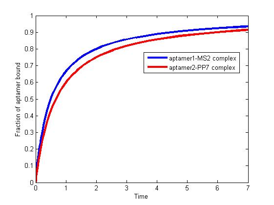
| | <p align="justify">We solve the differential equations numerically using the "ode" solver in Matlab. Titolo et at once come up with an approach to determine the equilibrium dissociation constant. This constant is dependent on anisotropies of the sample, aptamer, and intensities of the polarizers[1]. Therefore, the association rate constant and dissociation rate constant are usually experimentally determined values. It is difficult for us to determine the constants precisely since they vary in terms of experimental environment. </p>According to literature, we assumed that</p> | | <p align="justify">We solve the differential equations numerically using the "ode" solver in Matlab. Titolo et at once come up with an approach to determine the equilibrium dissociation constant. This constant is dependent on anisotropies of the sample, aptamer, and intensities of the polarizers[1]. Therefore, the association rate constant and dissociation rate constant are usually experimentally determined values. It is difficult for us to determine the constants precisely since they vary in terms of experimental environment. </p>According to literature, we assumed that</p> |
| Line 665: |
Line 432: |
| | <p align="justify"> </p> | | <p align="justify"> </p> |
| | <p align="justify">The results are shown as follows:</p> | | <p align="justify">The results are shown as follows:</p> |
| - | <div><img src="http://www.jiajunlu.com/igem/zju_model3_1.jpg"></div> | + | <div class="floatC"><img src="http://www.jiajunlu.com/igem/zju_model3_1.jpg"></div> |
| - | <p align="justify">Figure 1. The fraction of aptamer1-MS2 complex and the fraction of aptamer2-PP7 complex are increasing and finally reach equilibrium. </p> | + | <p class="fig" align="justify"><b>Fig 1.</b> The fraction of aptamer1-MS2 complex and the fraction of aptamer2-PP7 complex are increasing and finally reach equilibrium. </p> |
| | <p align="justify"> </p> | | <p align="justify"> </p> |
| | <p align="justify">As we mentioned above, the binding of MS2 to aptamer1 and the binding of PP7 to aptamer2 are independent with each other. The binding of one would not affect the binding of the other. From probability theoretical perspective, the fraction of RNA scaffold binding with both MS2 and PP7 is equal to the fraction of RNA scaffold binding with MS2 multiply the fraction of RNA scaffold binding with PP7. The RNA scaffold binding with both MS2 and PP7 is what we need to improve the reaction rate of pathways. </p> | | <p align="justify">As we mentioned above, the binding of MS2 to aptamer1 and the binding of PP7 to aptamer2 are independent with each other. The binding of one would not affect the binding of the other. From probability theoretical perspective, the fraction of RNA scaffold binding with both MS2 and PP7 is equal to the fraction of RNA scaffold binding with MS2 multiply the fraction of RNA scaffold binding with PP7. The RNA scaffold binding with both MS2 and PP7 is what we need to improve the reaction rate of pathways. </p> |
| | <p align="justify"> </p> | | <p align="justify"> </p> |
| - | <h3>References</h3> | + | <h2>References</h2> |
| - | <p align="justify">[1] Ajish S. R. Potty, Katerina Kourentzi, Han Fang, George W. Jackson, Xing Zhang, Glen B. Legge, Richard C. Willson. Biophysical Characterization of DNA Aptamer Interactions with Vascular Endothelial Growth Factor. 2008.</p> | + | <p class="ref" align="justify">[1] Ajish S. R. Potty, Katerina Kourentzi, Han Fang, George W. Jackson, Xing Zhang, Glen B. Legge, Richard C. Willson. Biophysical Characterization of DNA Aptamer Interactions with Vascular Endothelial Growth Factor. 2008.</p> |
| | + | </div> |
| | </div><!-- end .acc_container --> | | </div><!-- end .acc_container --> |
| | | | |
 "
"