Team:TU Darmstadt/Modeling MD

Molecular Dynamics

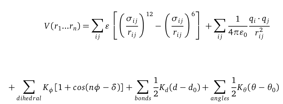
Molecular dynamics (MD) is one of the most common tools in computational biology. MD simulations solve the classical newton’s equations of motion. For the computation we need to calculate all forces acting in our system. The Forces are described within a potential energy -the Force Field and depends on the atomic coordinates r. For the illustration the potential is computed as follows:

The first term represents a a Lennard-Jones (LJ) potential. It approximates the interaction between a pair of neutral atoms or molecules. The second term is a coulomb potential between a pair of atom I and j. The last terms describe bonds and angles potentials. Due to experimental data and quantum chemical calculations the force-field parameters can be identified.The quality of MD simulations is mainly depending on the applied force field. In physics, a force field is a vector field which describes range dependent all non-contact forces acting on a particle. Applied in biochemistry a force field is a collection of mathematical functions and parameters which describe the potential energy of particles (atoms and molecules) in a defined system. For our simulations we used the AMBER (Assisted Model Building with Energy Refinement) force field which was especially developed to describe proteins and DNA.

Goal

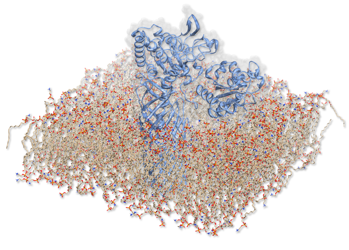
In order to characterize the enzyme construct and to simulate its complex behavior, MD was required to study the interactions. Hence to the degradation of PET, our Team designed a sophisticated protein-construct. This construct is a fusion protein containing a degradation module (PDB :1CEX, pnB) and EstA (PDB id: 3KVN), a membrane bounded beta-beryl. Moreover, this construct is exposed at the outer membrane of our bacteria. Hence, we quantified the dynamic nature of our degradation protein with coarse-grained methods we have to quantify the motion within this construct surrounded by its native environment. We firts have to create a scene were we put our fusion protein and put it into a membran layer. Although simulating this fusion protein was indispensable, it seems to be a complicated task.

Protocols

We used Yasara Structure simulation protocol for membrane protein. But we changed parameters and settings to fit it with our fusion protein-construct.

Analytics

RMSF

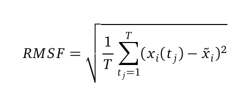
The Root mean square fluctuation (short: RMSF) can be computed as followed:

where T is the duration of the simulation (time steps) and xi(tj) the coordinates of atom xi at time tj. Now we are calculating the sum of the squared difference of the mean coordinate xi and xi(tj) . Furthermore we divide the sum to T and extract the root of it. Hence we are able to calculate the fluctuation of an atom with its mean in trajectory files. The RMSF was computed from the atomic coordinates of the C-alpha in R using the bio3d library.

RMSD

The Root mean square deviation (short: RMSF) can be computed as followed:

where n is the number of atoms (C-alpha or backbone atoms). Vi is defined as the coordinates of protein V atom I. Here, the RMSD is used to quantify a comparison between the structures of two protein (v and w) folds .The RMSD was computed from the atomic coordinates of the C-alpha in R using the bio3d library.