Team:TU Darmstadt/Modeling GNM

Homology Modeling |	Gaussian Networks |	Molecular Dynamics |	Information Theory |	Docking Simulation

---

Contents 1 Gaussian network model 1.1 Theory 1.2 Computation 1.2.1 Application to our Proteins 1.3 Results 1.3.1 References

Gaussian network model

Theory

Nearly all biologically important processes such as enzyme catalysis, ligand binding and allosteric regulation occur on a large time-scale (micro- to millisecond). A Gaussian network model (GNM) is a coarse-grained representation of a protein as a network consisting of balls and springs. In our approach, the protein chain is reduced to the coordinates of the C_α atom of each residue, represented by a ball. The springs simulate the connection between the amino acids. While Molecular Dynamics (MD) simulations are computational expensive, a GNM calculation only needs a few seconds.

Computation

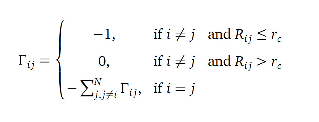
The dynamics of the structure in the GNM is described by the topology of contacts within the Kirchhoff matrix G. Thus in this network of N interacting sites, the elements of G are computed as:

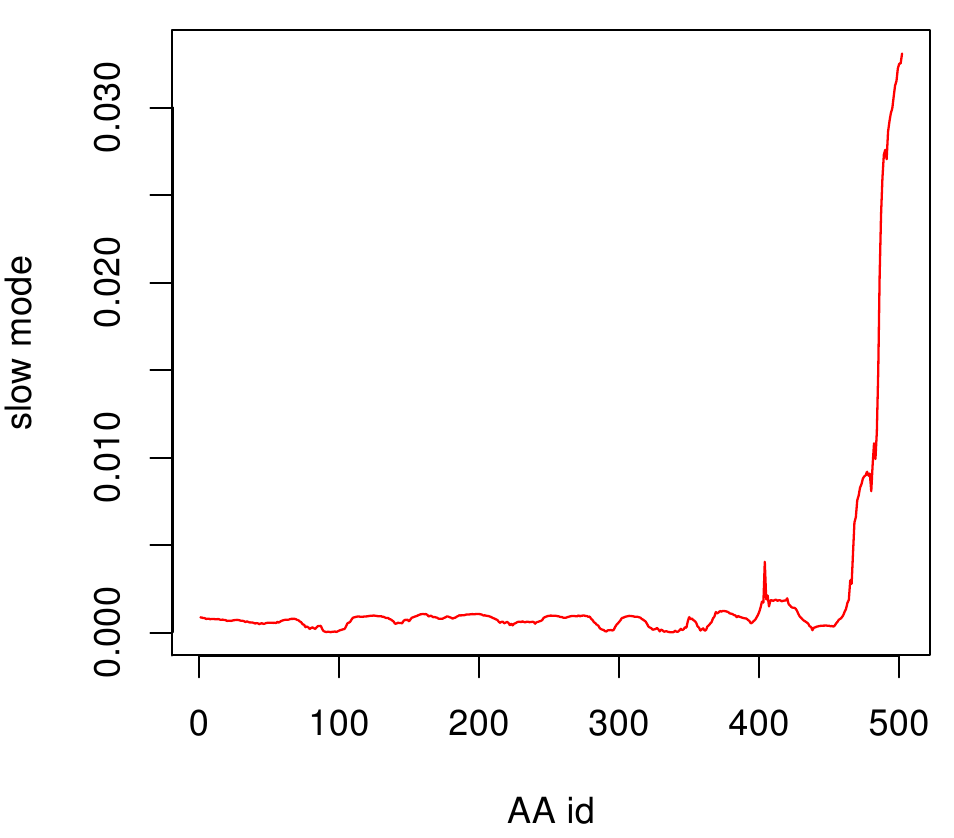
where R_ij is the distance between point i and j. We used Gamma as the intra C_α-contact matrix. The inverse of it describes correlations between fluctuations within the proteins native state. The diagonal of the matrix is replaced by the sum of contacts of one C_α-atom within the whole protein. After a singular value decomposition (SVD) we have calculated the normal modes of the protein. Slow modes describe functionally relevant residues within a biomolecule[2]⁠. The opposite, Fast modes, represent an uncorrelated motion without significant changes in the structure.

A recent examination of the X-ray crystallographic B-factors of over 100 proteins showed that the GNM closely reproduces the experimental data [3]⁠.

Application to our Proteins

We computed the GNM in R [4]⁠ by using the BioPhysConnectoR [5]⁠ library.

• PnB-Esterase 13
• AroY
• TpHA1
• TpHA2
• TpHA3

Results

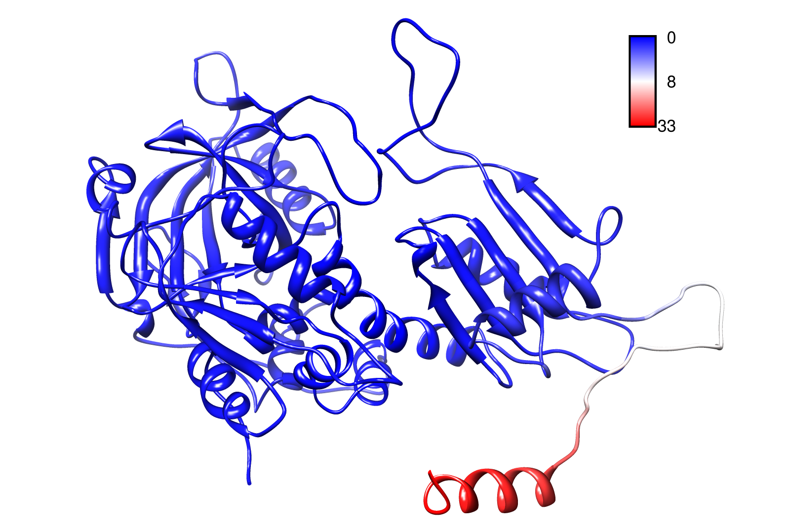
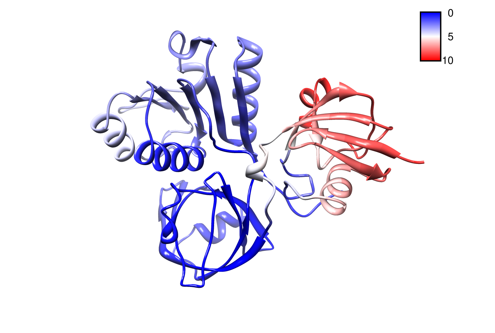
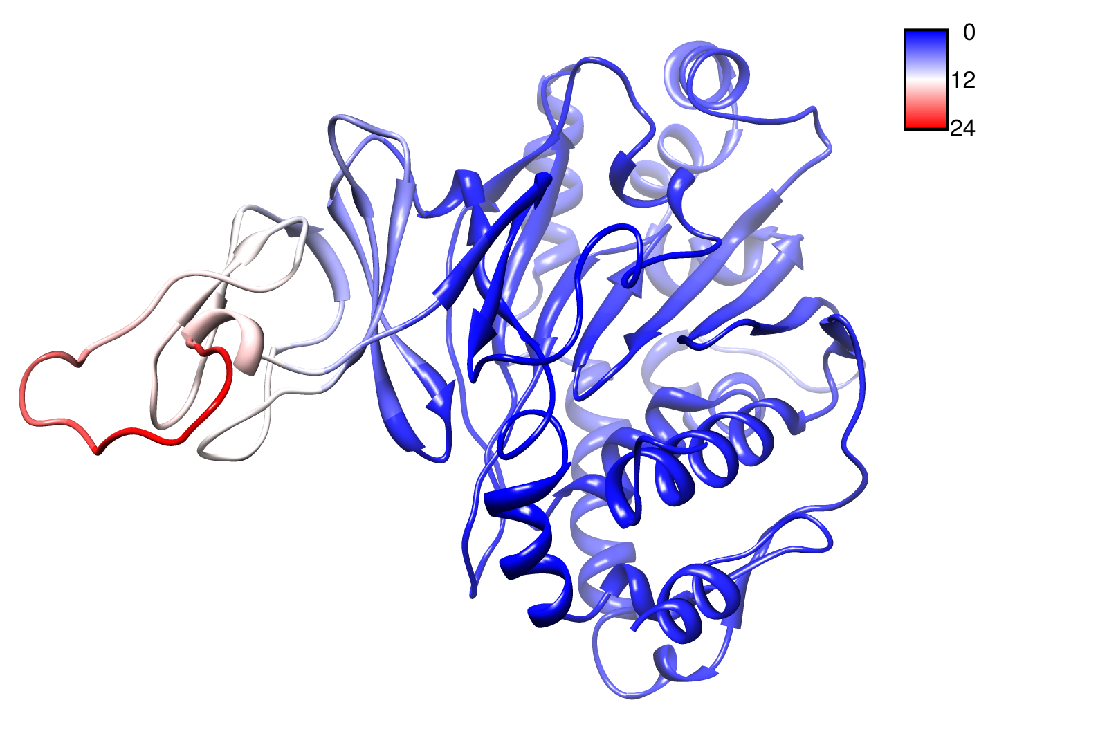
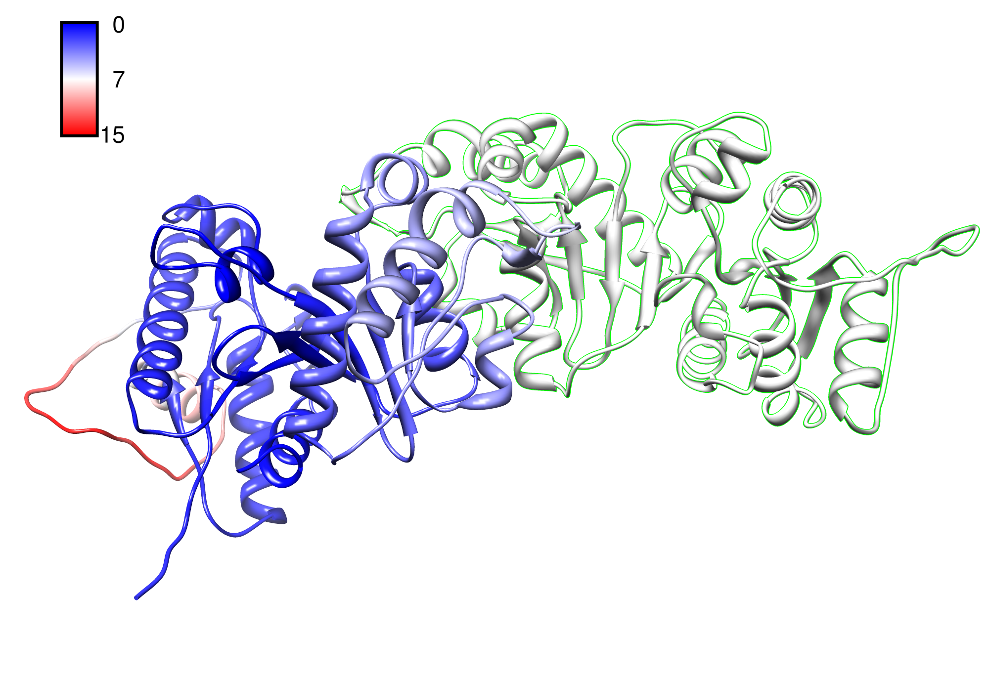
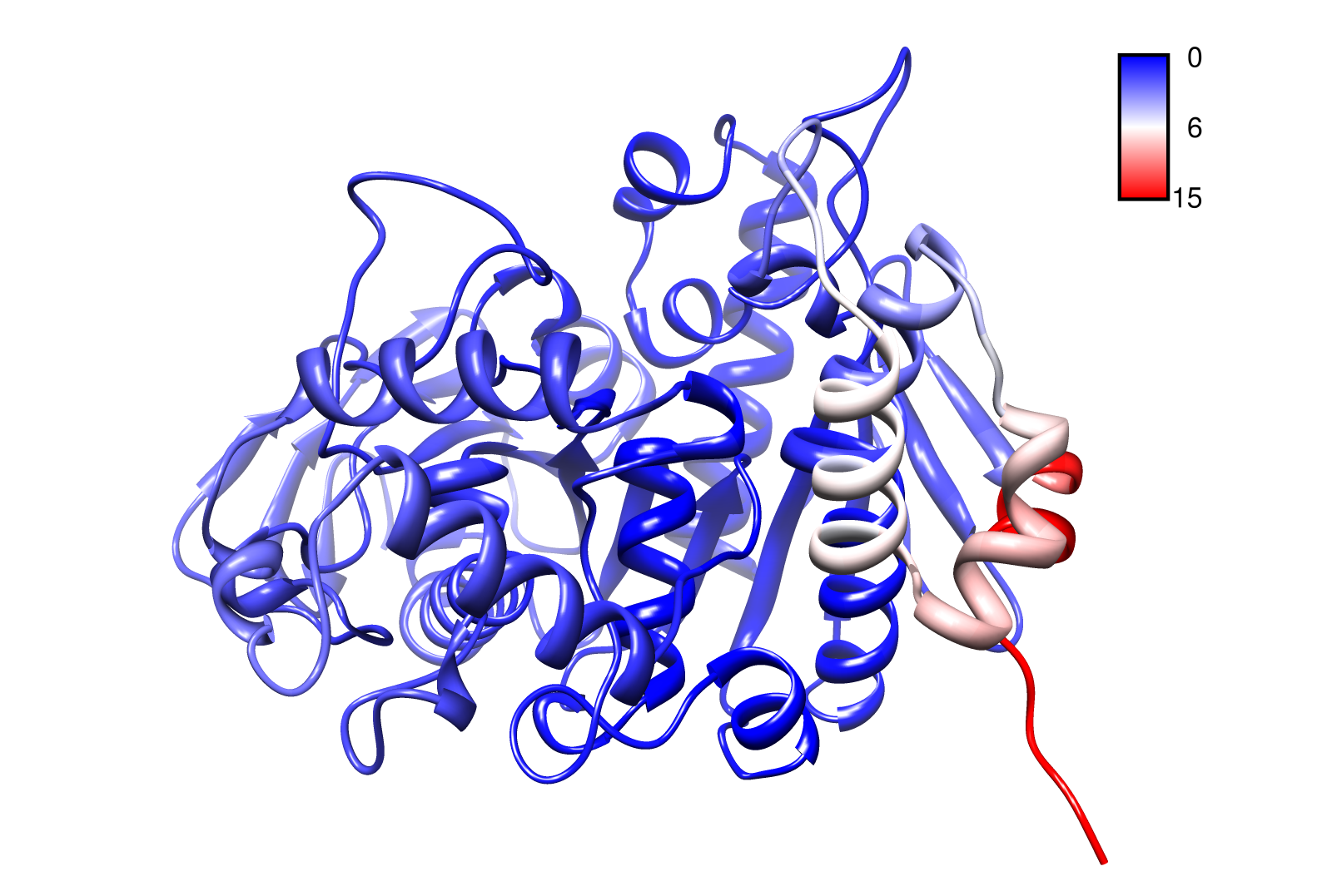
For the visualisation of the slow modes we colour coated the molcule structures. That actually means we replaced the atomic b-factors in our pdb files and substituted them with the slow mode values. Hence we are able to plot a heat-map on our protein structure.

• AroY

500px|left

500px|right

• TpHA3

• TpHA2

• TpHB

• PnB-Esterase 13

References

[1] A. R. Atilgan, S. R. Durell, R. L. Jernigan, M. C. Demirel, O. Keskin, and I. Bahar, “Anisotropy of fluctuation dynamics of proteins with an elastic network model.,” Biophys J, vol. 80, no. 1, pp. 505–515, Jan. 2001.

[2] C. Chennubhotla, A. J. Rader, L.-W. Yang, and I. Bahar, “Elastic network models for understanding biomolecular machinery: from enzymes to supramolecular assemblies.,” Physical Biology, vol. 2, no. 4, pp. S173–S180, 2005.

[3] I. Bahar and A. J. Rader, “Coarse-grained normal mode analysis in structural biology.,” Current Opinion in Structural Biology, vol. 15, no. 5, pp. 586–592, 2005.

[4] R. D. C. Team, “R: A Language and Environment for Statistical Computing.” Vienna, Austria, 2008.

[5] F. Hoffgaard, P. Weil, and K. Hamacher, “BioPhysConnectoR: Connecting sequence information and biophysical models.,” BMC Bioinformatics, vol. 11, p. 199, 2010.