"
"
Team:Carnegie Mellon/Mod-Derivations
From 2012.igem.org
| (86 intermediate revisions not shown) | |||
| Line 5: | Line 5: | ||
<!-- Nav Bar --> | <!-- Nav Bar --> | ||
| - | |||
<ul class="sf-menu sf-navbar"> | <ul class="sf-menu sf-navbar"> | ||
<li style ='width: 193px'> | <li style ='width: 193px'> | ||
| Line 20: | Line 19: | ||
</li> | </li> | ||
<li> | <li> | ||
| - | <a href="https://2012.igem.org/Team:Carnegie_Mellon/Hom- | + | <a href="https://2012.igem.org/Team:Carnegie_Mellon/Hom-Attributions">Attributions</a> |
| + | </li> | ||
| + | <li> | ||
| + | <a href="https://2012.igem.org/Team:Carnegie_Mellon/Hom-Acknowledgements">Acknowledgements</a> | ||
</li> | </li> | ||
</ul> | </ul> | ||
| Line 33: | Line 35: | ||
<li> | <li> | ||
<a href="https://2012.igem.org/Team:Carnegie_Mellon/Bio-Submitted">Submitted Parts</a> | <a href="https://2012.igem.org/Team:Carnegie_Mellon/Bio-Submitted">Submitted Parts</a> | ||
| - | |||
| - | |||
| - | |||
</li> | </li> | ||
</ul> | </ul> | ||
| Line 58: | Line 57: | ||
<li> | <li> | ||
<a href="https://2012.igem.org/Team:Carnegie_Mellon/Met-Notebook">Notebook</a> | <a href="https://2012.igem.org/Team:Carnegie_Mellon/Met-Notebook">Notebook</a> | ||
| + | </li> | ||
| + | <li> | ||
| + | <a href="https://2012.igem.org/Team:Carnegie_Mellon/Met-Safety">Safety</a> | ||
| + | </li> | ||
</ul> | </ul> | ||
</li> | </li> | ||
| - | <li class="current" | + | <li class="current" style ='width: 193px'> |
<a href="https://2012.igem.org/Team:Carnegie_Mellon/Mod-Overview">Modeling</a> | <a href="https://2012.igem.org/Team:Carnegie_Mellon/Mod-Overview">Modeling</a> | ||
<ul> | <ul> | ||
| Line 73: | Line 76: | ||
<li> | <li> | ||
<a href="https://2012.igem.org/Team:Carnegie_Mellon/Mod-Matlab">Matlab</a> | <a href="https://2012.igem.org/Team:Carnegie_Mellon/Mod-Matlab">Matlab</a> | ||
| + | </li> | ||
| + | <li> | ||
| + | <a href="https://2012.igem.org/Team:Carnegie_Mellon/Mod-Expanded">Expanded</a> | ||
</li> | </li> | ||
</ul> | </ul> | ||
| Line 80: | Line 86: | ||
<a href="https://2012.igem.org/Team:Carnegie_Mellon/Hum-Overview">Human Practices</a> | <a href="https://2012.igem.org/Team:Carnegie_Mellon/Hum-Overview">Human Practices</a> | ||
<ul> | <ul> | ||
| - | <li class = 'offset' style ='width: | + | <li class = 'offset' style ='width: 302px'> <a href="#"></a></li> |
<li> | <li> | ||
<a href="https://2012.igem.org/Team:Carnegie_Mellon/Hum-Overview">Overview</a> | <a href="https://2012.igem.org/Team:Carnegie_Mellon/Hum-Overview">Overview</a> | ||
| Line 89: | Line 95: | ||
<li> | <li> | ||
<a href="https://2012.igem.org/Team:Carnegie_Mellon/Hum-Circuit">Circuit Kit</a> | <a href="https://2012.igem.org/Team:Carnegie_Mellon/Hum-Circuit">Circuit Kit</a> | ||
| - | + | </li> | |
| - | + | <li> | |
| - | + | <a href="https://2012.igem.org/Team:Carnegie_Mellon/Hum-Software">Software</a> | |
| - | + | </li> | |
| - | + | <li> | |
| - | + | <a href="https://2012.igem.org/Team:Carnegie_Mellon/Hum-Team">Team Presentation</a> | |
| - | + | </li> | |
| - | </ | + | <li> |
| + | <a href="https://2012.igem.org/Team:Carnegie_Mellon/Hum-Teaching">Teaching Presentation</a> | ||
</li> | </li> | ||
</ul> | </ul> | ||
| Line 102: | Line 109: | ||
</ul> | </ul> | ||
<br /><br /><br /> | <br /><br /><br /> | ||
| + | |||
| Line 134: | Line 142: | ||
<body> | <body> | ||
<h1 id = "section1-1">Documentation Preface</h1> | <h1 id = "section1-1">Documentation Preface</h1> | ||
| - | <p>The documentation of the model consists of the derivations of all the equations used to create the model. Each equation contributes a piece of the picture which ultimately results in the calculations of important cell characteristics. These equations live in the | + | <p>The documentation of the model consists of the derivations of all the equations used to create the model. Each equation contributes a piece of the picture which ultimately results in the calculations of important cell characteristics. These equations live in the Matlab model that can be found <a rel="external" href="https://2012.igem.org/Team:Carnegie_Mellon/Mod-Matlab">here</a>. |
| - | The characteristics we are measuring include transcriptional | + | The characteristics we are measuring include transcriptional strength, <i>Ts </i> \eqref{eq:eR}, translational efficiency, <i>Tl </i> \eqref{eq:Tl}, and Polymerase Per Second, <i> PoPS</i> \eqref{eq:PoPS}. |
</p> | </p> | ||
| - | Note: | + | Note: We derived equations for the model to fit the data that we obtained experimentally, while the Matlab code has even broader application and can be applied to several different experimental setups (e.g., measurement of fluorescence of both RNA and protein in the presence of degradation only, or both synthesis and degradation). These equations formed the foundation that helped extract some important cellular characteristics from the raw data that we took. |
| - | <h1 id = "section1-2" | + | <br /> |
| + | <br /> | ||
| + | |||
| + | <h1 id = "section1-2">Experimental Data Analysis</h1> | ||
| + | <br /> | ||
<p> | <p> | ||
| - | Let fluorescent mRNA and protein concentration be represented by $[R_f]$ and $[P_f]$ respectively. They are related directly to the fluorescence level, which we will label $F_r$ and $F_p$. | + | Let fluorescent mRNA and protein concentration (concentration of the mRNA/dye and protein/dye complexes) be represented by $[R_f]$ and $[P_f]$, respectively. They are related directly to the fluorescence level, which we will label $F_r$ and $F_p$. Thus, we can write |
</p> | </p> | ||
| Line 149: | Line 161: | ||
<p> | <p> | ||
| - | + | where $S_r$ and $S_p$ are scaling factors for mRNA and protein, respectively, and $k_r$ and $k_p$ are constants that transform fluorescence to mRNA and protein concentrations. | |
</p> | </p> | ||
| Line 155: | Line 167: | ||
In the experiment, one uses a plate reader with varying concentration of the dyes in rows and varying time measurements in columns. The following image represents this. | In the experiment, one uses a plate reader with varying concentration of the dyes in rows and varying time measurements in columns. The following image represents this. | ||
</p> | </p> | ||
| - | + | <img src = "https://static.igem.org/mediawiki/2012/0/0f/DyePicture.png" height = "400" width = "350" > | |
<p> | <p> | ||
| - | We will also have another row for in vitro measurements. From this row we will graph the fluorescence versus the dye concentration, and the fluorescence will level off at some saturation point. Because the saturation point in vitro will be greater than the saturation point in vivo, we must scale all the fluorescence measurements we find in vivo, which is the importance of $S_r$ and $S_p$. | + | We will also have another row for <i> in vitro</i> measurements. From this row we will graph the fluorescence versus the dye concentration, and the fluorescence will level off at some saturation point. Because the saturation point <i> in vitro</i> will be greater than the saturation point <i> in vivo</i>, we must scale all the fluorescence measurements we find <i> in vivo </i>, which is the importance of $S_r$ and $S_p$. |
</p> | </p> | ||
<p> | <p> | ||
| - | At this point we will find out the scaling factors $S_r$ and $S_p$. Step 1 is to put samples into the plate reader and take more samples of the same concentration and measure them in vitro. Then, we will measure all the wells at the same time point, and find the saturation fluorescence of the in vitro and the in vivo wells. Dividing the two gives us the $S_r$ and $S_p$. | + | At this point we will find out the scaling factors $S_r$ and $S_p$. Step 1 is to put samples into the plate reader and take more samples of the same concentration and measure them <i> in vitro</i>. Then, we will measure all the wells at the same time point, and find the saturation fluorescence of the <i> in vitro</i> and the <i> in vivo </i> wells. Dividing the two gives us the $S_r$ and $S_p$. |
</p> | </p> | ||
<p> | <p> | ||
| - | At each time point we will graph the in vivo fluorescence vs dye concentrations and find the first dye concentration where saturation occurs. This dye concentration is thus the mRNA/protein total concentration, as we will assume that there will be a 1-1 correspondence of dye and mRNA/protein. We then multiply each by the scaling factor $S_r$ or $S_p$ to get the actual mRNA. | + | At each time point we will graph the <i> in vivo </i> fluorescence vs. dye concentrations and find the first dye concentration where saturation occurs. This dye concentration is thus the mRNA/protein total concentration, as we will assume that there will be a 1-1 correspondence of dye and mRNA/protein. We then multiply each by the scaling factor $S_r$ or $S_p$ to get the actual mRNA. |
</p> | </p> | ||
| + | <br\> | ||
| + | |||
<h1 id = "section1-3">Equilibrium Constants</h1> | <h1 id = "section1-3">Equilibrium Constants</h1> | ||
<br /><br /> | <br /><br /> | ||
| Line 173: | Line 187: | ||
\begin{equation}\alpha [A] + \beta [B] \leftrightarrow \gamma [AB]\end{equation} | \begin{equation}\alpha [A] + \beta [B] \leftrightarrow \gamma [AB]\end{equation} | ||
<p> | <p> | ||
| - | + | where $\alpha$, $\beta$, $\gamma$ are coefficients describing the ratio of molecules of $[A]$ and $[B]$ needed to synthesize $[AB]$. $[A]$, $[B]$, and $[AB]$ are different molecule concentrations. After some time, there will be some equilibrium where some amount of $[A]$ and $[B]$ become $[AB]$. So then, the equation at equilibrium becomes: | |
</p> | </p> | ||
<p> | <p> | ||
| - | \begin{equation}(\alpha[A] - \gamma [AB]) + (\beta[B] - \gamma [AB]) \leftrightarrow \gamma [AB]\end{equation} | + | \begin{equation}(\alpha[A] - \gamma [AB]) + (\beta[B] - \gamma [AB]) \leftrightarrow \gamma [AB]\label{eq:equi}\end{equation} |
</p> | </p> | ||
<p> | <p> | ||
| - | We will assume that $\alpha$, $\beta$, and $\gamma$ are all equal to 1. Our $[A]$ will be mRNA/protein and $[B]$ will be the dye concentrations. mRNA dye, which is DFHBI, will be $[ | + | We will assume that $\alpha$, $\beta$, and $\gamma$ are all equal to 1. Our $[A]$ will be mRNA/protein and $[B]$ will be the dye concentrations. mRNA dye, which is DFHBI, will be $[D_R]$ and protein dye, which is malachite green (MG), will be $[D_P]$. $[R]_0$ and $[P]_0$ are the initial concentrations of RNA and protein, respectively. Our equations are thus: |
</p> | </p> | ||
<p> | <p> | ||
| - | \begin{equation}([R] | + | \begin{equation}([R]_0 - [R_f]) + ([D_R] - [R_f]) \leftrightarrow ([R_f])\end{equation} |
| - | \begin{equation}([P] | + | \begin{equation}([P]_0 - [P_f]) + ([D_P] - [P_f]) \leftrightarrow ([P_f])\end{equation} |
</p> | </p> | ||
<p> | <p> | ||
| - | + | The equilibrium constant for RNA, $K_{D_R}$ is then defined as the product of the reaction product concentrations over the reactant concentrations. We will take the equilibrium constant at equilibrium, so from equation \eqref{eq:equi}, we can determine the equilibrium constant. We will have $[A]_0$ and $[B]_0$ instead of $[A]$ and $[B]$ to signify the initial concentrations of $[A]$ and $[B]$. | |
</p> | </p> | ||
| - | \begin{equation}K_{D_R} = \frac{[AB]}{([A]_0 - [AB]) ([B]_0 - [AB])}\end{equation} | + | \begin{equation}K_{D_R} = \frac{[AB]}{([A]_0 - [AB]) ([B]_0 - [AB])}\end{equation} |
<p> | <p> | ||
| - | Now inputting our variables for mRNA expression, | + | Now inputting our variables for mRNA expression, once again using $[R]_0$ and $[D_R]_0$ to signify initial concentration of $[R]$ and $[D_R]$: |
</p> | </p> | ||
<p> | <p> | ||
| Line 197: | Line 211: | ||
</p> | </p> | ||
<p> | <p> | ||
| - | + | we can solve for $[Rf]$ using a quadratic equation based off of \eqref{eq:8}. | |
</p> | </p> | ||
<p> | <p> | ||
\begin{equation}[R_f]^2 \cdot K_{D_R} - [R_f]\cdot [K_{D_R}([R] + D_R) + 1] + K_{D_R} \cdot [R] \cdot {D_R} = 0\end{equation} | \begin{equation}[R_f]^2 \cdot K_{D_R} - [R_f]\cdot [K_{D_R}([R] + D_R) + 1] + K_{D_R} \cdot [R] \cdot {D_R} = 0\end{equation} | ||
</p> | </p> | ||
| - | \begin{equation}[R_f] = \frac{[K_{D_R}([R][D_R]) + 1] \pm \sqrt{[K_{D_R}([R][D_R]) + 1]^2 - 4 \cdot (K_{D_R}) \cdot (K_{D_R}[R][D_R])}}{2 \cdot K_{D_R}}\end{equation} | + | \begin{equation}[R_f] = \frac{[K_{D_R}([R][D_R]) + 1] \pm \sqrt{[K_{D_R}([R][D_R]) + 1]^2 - 4 \cdot (K_{D_R}) \cdot (K_{D_R}[R][D_R])}}{2 \cdot K_{D_R}}\end{equation} |
<p> | <p> | ||
| - | + | We can apply the similar procedure for determining the protein concentration. | |
</p> | </p> | ||
<p> | <p> | ||
</p> | </p> | ||
| - | + | <br /> | |
| + | <h1 id = "section1-4">Degradation</h1> | ||
| + | <br /> | ||
<p> | <p> | ||
Degradation occurs for both mRNA and protein. After shutting off production of mRNA/protein, one can measure the degradation coefficient. Some intuition | Degradation occurs for both mRNA and protein. After shutting off production of mRNA/protein, one can measure the degradation coefficient. Some intuition | ||
| - | reveals that the amount that is degraded is proportional to the amount of mRNA/protein that is present. | + | reveals that the amount that is degraded is proportional to the amount of mRNA/protein that is present. We will let $\frac{d[R]_D}{dt}$ be the change in the concentration of RNA, and $\alpha$ be the degradation coefficient determining the fraction of RNA that will be degraded in time. |
</p> | </p> | ||
<p> | <p> | ||
| - | \begin{equation}\frac{d[R]}{dt} = -\alpha \cdot [R]\end{equation} | + | \begin{equation}\frac{d[R]_D}{dt} = -\alpha \cdot [R]\end{equation} |
</p> | </p> | ||
<p> | <p> | ||
Protein often has another constant attached to degradation, labeled maturation. Maturation $(a)$ takes into account the time it takes for a protein to | Protein often has another constant attached to degradation, labeled maturation. Maturation $(a)$ takes into account the time it takes for a protein to | ||
| - | mature before fluorescence can actually occur. Maturation is also dependent on the amount of protein available. In this case, the equation would be | + | mature before fluorescence can actually occur. Maturation is also dependent on the amount of protein available. We will let $\frac{d[P]_D}{dt}$ be the change in the concentration of protein, and $\beta$ be the degradation coefficient determining the fraction of protein that will be degraded in time. In this case, the equation would be |
</p> | </p> | ||
<p> | <p> | ||
| - | \begin{equation}\frac{d[P]}{dt} = -(a + \beta) \cdot [P]\label{eq:12}\end{equation} | + | \begin{equation}\frac{d[P]_D}{dt} = -(a + \beta) \cdot [P]\label{eq:12}\end{equation} |
</p> | </p> | ||
<p> | <p> | ||
However, since the fluorogen activated protein (FAP) takes a small amount of time to fold and to bind to the dye, one can make a reasonable assumption that | However, since the fluorogen activated protein (FAP) takes a small amount of time to fold and to bind to the dye, one can make a reasonable assumption that | ||
| - | maturation is 0. So the simplified equation is | + | maturation is 0. So the simplified equation is: |
</p> | </p> | ||
<p> | <p> | ||
| - | \begin{equation}\frac{d[P]}{dt} = -\beta \cdot [P] \label{eq:13}\end{equation} | + | \begin{equation}\frac{d[P]}{dt} = -\beta \cdot [P] \label{eq:13}\end{equation} |
</p> | </p> | ||
<p> | <p> | ||
| - | Equations \eqref{eq:12} and \eqref{eq:13} can be solved by first order linear differential equation techniques. | + | Equations \eqref{eq:12} and \eqref{eq:13} can be solved by first order linear differential equation techniques. We will let $[R]_{max}$ and $[P]_{max}$ be the theoretical maximum concentration of RNA and protein (can also be thought of as at equilibrium): |
</p> | </p> | ||
<p> | <p> | ||
\begin{equation}[R] = [R]_{max}\cdot e^{-\alpha \cdot t}\end{equation} | \begin{equation}[R] = [R]_{max}\cdot e^{-\alpha \cdot t}\end{equation} | ||
| - | \begin{equation}[P] = [P]_{max}\cdot e^{-\beta \cdot t}\end{equation} | + | \begin{equation}[P] = [P]_{max}\cdot e^{-\beta \cdot t}\end{equation} |
</p> | </p> | ||
<p> | <p> | ||
| Line 243: | Line 259: | ||
</p> | </p> | ||
| - | <h1 id = "section1-5" | + | <br /> |
| + | <h1 id = "section1-5" >mRNA Expression</h1> | ||
| + | <br /> | ||
<p> | <p> | ||
| Line 252: | Line 270: | ||
</p> | </p> | ||
<p> | <p> | ||
| - | + | where $Ts$ is the transcriptional efficiency and $\alpha$ is the degradation constant associated with mRNA degradation, $\frac{d[R]}{dt}$ is the change in RNA over time, and $[R]$ is the mRNA concentration or amount. | |
</p> | </p> | ||
<p> | <p> | ||
| Line 258: | Line 276: | ||
</p> | </p> | ||
<p> | <p> | ||
| - | \begin{equation}\frac{d[R]}{dt} + \alpha \cdot [R] = Ts \cdot [D] \label{eq:e1}\end{equation} | + | \begin{equation}\frac{d[R]}{dt} + \alpha \cdot [R] = Ts \cdot [D] \label{eq:e1}\end{equation} |
</p> | </p> | ||
<p> | <p> | ||
| - | The small integrating factor is thus $e^{\alpha \cdot t}$ | + | The small integrating factor is thus $e^{\alpha \cdot t}$. |
</p> | </p> | ||
<p> | <p> | ||
| Line 279: | Line 297: | ||
<p> | <p> | ||
| - | At $t = 0$, $[R] = 0$. Plugging into \eqref{eq:e2} | + | At $t = 0$, $[R] = 0$. Plugging into \eqref{eq:e2}, we obtain: |
</p> | </p> | ||
| Line 288: | Line 306: | ||
\begin{equation}[R] = \frac{Ts \cdot [D]}{\alpha} - \frac{Ts \cdot [D]}{\alpha} \cdot e^{-\alpha \cdot t}\end{equation} | \begin{equation}[R] = \frac{Ts \cdot [D]}{\alpha} - \frac{Ts \cdot [D]}{\alpha} \cdot e^{-\alpha \cdot t}\end{equation} | ||
| - | \begin{equation}[R] = \frac{Ts \cdot [D]}{\alpha} \cdot (1 - e^{-\alpha \cdot t})\label{eq:eR}\end{equation} | + | \begin{equation}[R] = \frac{Ts \cdot [D]}{\alpha} \cdot (1 - e^{-\alpha \cdot t})\label{eq:eR}\end{equation} |
<p> | <p> | ||
| Line 294: | Line 312: | ||
</p> | </p> | ||
| - | \begin{equation} Ts = \frac{[R] \cdot \alpha}{[D] \cdot (1 - e^{-\alpha \cdot t})}\end{equation} | + | \begin{equation} Ts = \frac{[R] \cdot \alpha}{[D] \cdot (1 - e^{-\alpha \cdot t})}\end{equation} |
</p> | </p> | ||
| + | <br /> | ||
| - | <h1 id = "section1-6" | + | <h1 id = "section1-6">Protein Expression</h1> |
| - | + | <br /> | |
<p> | <p> | ||
The protein model is a bit different from the mRNA model due to the fact that the amount of protein depends on the amount of mRNA, which is variable. mRNA | The protein model is a bit different from the mRNA model due to the fact that the amount of protein depends on the amount of mRNA, which is variable. mRNA | ||
| Line 310: | Line 329: | ||
<p> | <p> | ||
| - | + | where $[P]$ is the protein concentration or amount, $[R]$ is still mRNA, $Tl$ is the translational efficiency, and $\beta$ is the degradation constant associated | |
with the protein. | with the protein. | ||
</p> | </p> | ||
<p> | <p> | ||
| - | Conveniently, we have already solved for our only hurdle to a first order linear equation, the mRNA amount (from equation \eqref{eq:eR}). We will substitute in for mRNA now | + | Conveniently, we have already solved for our only hurdle to a first order linear equation, the mRNA amount (from equation \eqref{eq:eR}). We will substitute in for mRNA now: |
</p> | </p> | ||
<p> | <p> | ||
| - | \begin{equation}\frac{d[P]}{dt} = (1 - e^{-\alpha \cdot t}) \cdot \frac{Ts \cdot [D]}{\alpha} \cdot Tl - \beta \cdot [P]\end{equation} | + | \begin{equation}\frac{d[P]}{dt} = (1 - e^{-\alpha \cdot t}) \cdot \frac{Ts \cdot [D]}{\alpha} \cdot Tl - \beta \cdot [P]\end{equation} |
</p> | </p> | ||
<p> | <p> | ||
| - | Now we can solve the first order linear equation | + | Now we can solve the first order linear equation: |
</p> | </p> | ||
<p> | <p> | ||
| - | \begin{equation}\frac{d[P]}{dt} + \beta \cdot [P] = (1 - e^{-\alpha \cdot t}) \cdot \frac{Ts \cdot [D]}{\alpha} \cdot Tl\end{equation} | + | \begin{equation}\frac{d[P]}{dt} + \beta \cdot [P] = (1 - e^{-\alpha \cdot t}) \cdot \frac{Ts \cdot [D]}{\alpha} \cdot Tl\end{equation} |
</p> | </p> | ||
<p> | <p> | ||
| - | It can be seen that the integrating factor is $e^{\beta \cdot t}$ | + | It can be seen that the integrating factor is $e^{\beta \cdot t}$ : |
</p> | </p> | ||
\begin{equation}\frac{d[P]}{dt} \cdot e^{\beta \cdot t} + \beta \cdot [P] \cdot e^{\beta \cdot t} = e^{\beta \cdot t} \cdot (1 - e^{-\alpha \cdot t}) \cdot \frac{Ts \cdot [D]}{\alpha} \cdot Tl\end{equation} | \begin{equation}\frac{d[P]}{dt} \cdot e^{\beta \cdot t} + \beta \cdot [P] \cdot e^{\beta \cdot t} = e^{\beta \cdot t} \cdot (1 - e^{-\alpha \cdot t}) \cdot \frac{Ts \cdot [D]}{\alpha} \cdot Tl\end{equation} | ||
| Line 336: | Line 355: | ||
\begin{equation}[P]\cdot e^{\beta \cdot t} = Tl \cdot \int \! \frac{Ts \cdot [D]}{\alpha} \cdot e^{\beta \cdot t} \ dt - Tl \cdot \int \!\frac{Ts \cdot [D]}{\alpha} \cdot e^{(-\alpha + \beta) \cdot t} \ dt\end{equation} | \begin{equation}[P]\cdot e^{\beta \cdot t} = Tl \cdot \int \! \frac{Ts \cdot [D]}{\alpha} \cdot e^{\beta \cdot t} \ dt - Tl \cdot \int \!\frac{Ts \cdot [D]}{\alpha} \cdot e^{(-\alpha + \beta) \cdot t} \ dt\end{equation} | ||
| - | \begin{equation}[P] \cdot e^{\beta \cdot t} = Tl \cdot \frac{Ts \cdot [D]}{\alpha \cdot \beta} \cdot e^{\beta \cdot t} - Tl \cdot \frac{Ts \cdot [D]}{\alpha \cdot (-\alpha + \beta)} \cdot e^{(-\alpha + \beta) \cdot t} + C \label{eq:34}\end{equation} | + | \begin{equation}[P] \cdot e^{\beta \cdot t} = Tl \cdot \frac{Ts \cdot [D]}{\alpha \cdot \beta} \cdot e^{\beta \cdot t} - Tl \cdot \frac{Ts \cdot [D]}{\alpha \cdot (-\alpha + \beta)} \cdot e^{(-\alpha + \beta) \cdot t} + C \label{eq:34}\end{equation} |
<p> | <p> | ||
| - | Now we solve for C. When $t = 0$, $P = 0$ | + | Now we solve for C. When $t = 0$, $P = 0$ : |
</p> | </p> | ||
| - | \begin{equation}C = -Tl \cdot \frac{Ts \cdot [D]}{\alpha} \cdot (\frac{1}{\beta} - \frac{1}{-\alpha + \beta})\end{equation} | + | \begin{equation}C = -Tl \cdot \frac{Ts \cdot [D]}{\alpha} \cdot (\frac{1}{\beta} - \frac{1}{-\alpha + \beta})\end{equation} |
<p> | <p> | ||
| - | Substituting into \eqref{eq:34}: | + | Substituting into \eqref{eq:34}, we obtain: |
| - | \begin{equation}[P] \cdot e^{\beta \cdot t} = Tl \cdot \frac{Ts \cdot [D]}{\alpha \cdot \beta} \cdot e^{\beta \cdot t} - Tl \cdot \frac{Ts \cdot [D]}{\alpha \cdot (-\alpha + \beta)} \cdot e^{(-\alpha + \beta) \cdot t} - Tl \cdot \frac{Ts \cdot [D]}{\alpha} \cdot (\frac{1}{\beta} - \frac{1}{-\alpha + \beta}) \end{equation} | + | \begin{equation}[P] \cdot e^{\beta \cdot t} = Tl \cdot \frac{Ts \cdot [D]}{\alpha \cdot \beta} \cdot e^{\beta \cdot t} - Tl \cdot \frac{Ts \cdot [D]}{\alpha \cdot (-\alpha + \beta)} \cdot e^{(-\alpha + \beta) \cdot t} - Tl \cdot \frac{Ts \cdot [D]}{\alpha} \cdot (\frac{1}{\beta} - \frac{1}{-\alpha + \beta}) \end{equation} |
</p> | </p> | ||
<p> | <p> | ||
| Line 350: | Line 369: | ||
</p> | </p> | ||
<p> | <p> | ||
| - | FInally, we solve for Tl. Tl is the translational efficiency, which is the second characteristic we were trying to solve for | + | FInally, we solve for Tl. Tl is the translational efficiency, which is the second characteristic we were trying to solve for: |
</p> | </p> | ||
\begin{equation}Tl = \frac{[P]}{\frac{Ts \cdot [D]}{(\alpha \cdot \beta)} \cdot (1 - e^{-\beta \cdot t}) - \frac{Ts \cdot [D]}{\alpha \cdot (-\alpha + \beta)} \cdot (e^{-\alpha \cdot t} - e^{-\beta \cdot t})} \label{eq:Tl}\end{equation} | \begin{equation}Tl = \frac{[P]}{\frac{Ts \cdot [D]}{(\alpha \cdot \beta)} \cdot (1 - e^{-\beta \cdot t}) - \frac{Ts \cdot [D]}{\alpha \cdot (-\alpha + \beta)} \cdot (e^{-\alpha \cdot t} - e^{-\beta \cdot t})} \label{eq:Tl}\end{equation} | ||
| + | <br /> | ||
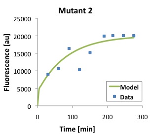
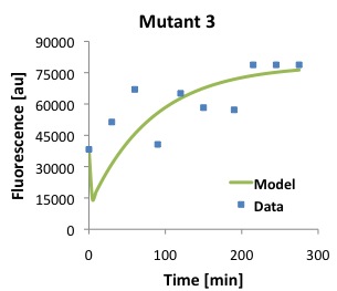
| + | <p> The following figures show that our model described above, and the parameters that we obtained fit well the measured fluorescence for the wild type (WT) promoter and three new promoters (Mutants 1,2, and 3). </p> | ||
| + | |||
| + | <p> | ||
| + | <img src="https://static.igem.org/mediawiki/2012/e/e1/WT.jpg" height="180" width="210" align="center"/> | ||
| + | |||
| + | <img src="https://static.igem.org/mediawiki/2012/1/10/Mutant1.jpg" height="180" width="210" align="center"/> | ||
| + | |||
| + | <img src="https://static.igem.org/mediawiki/2012/d/db/Mutant2.jpg" height="180" width="210" align="center"/> | ||
| + | |||
| + | <img src="https://static.igem.org/mediawiki/2012/8/86/Mutant3.jpg" height="180" width="210" align="center"/> | ||
| + | </p> | ||
| - | |||
| + | <h1 id = "section1-7">Polymerase Per Second</h1> | ||
| + | <br /> | ||
<p> | <p> | ||
| - | Taking inspiration from ”Measuring the activity of BioBrick promoters using an in vivo reference standard” by Kelly et al., we can derive our own equation | + | Taking inspiration from ”Measuring the activity of BioBrick promoters using an <i>in vivo</i> reference standard” by Kelly et al.<sup><a href = "#cite1">[1]</a></sup>, we can derive our own equation |
| - | for polymerase per second (PoPS). | + | for polymerase per second (PoPS), as follows. |
</p> | </p> | ||
<p> | <p> | ||
| - | mRNA is produced by the number of promoters times the rate of initiations of polymerase onto the promoters, or $n \cdot PoPS$. mRNA is degraded by the degradation equation we derived earlier, which is $-\alpha \cdot [R]$ | + | mRNA is produced by the number of promoters times the rate of initiations of polymerase onto the promoters, or $n \cdot PoPS$. mRNA is degraded by the degradation equation we derived earlier, which is $-\alpha \cdot [R]$ : |
</p> | </p> | ||
<p> | <p> | ||
| - | \begin{equation}\frac{d[R]}{dt} = n \cdot PoPS - \alpha \cdot [R] \label{eq:Po1}\end{equation} | + | \begin{equation}\frac{d[R]}{dt} = n \cdot PoPS - \alpha \cdot [R] \label{eq:Po1}\end{equation} |
</p> | </p> | ||
<p> | <p> | ||
| - | + | where $n$ is the number of promoters in a cell, PoPS is the rate of initiations of RNA polymerase onto the promoters. | |
</p> | </p> | ||
<p> | <p> | ||
| - | Protein is produced by the translational efficiency times the mRNA, which is $[R] \cdot Tl$. Protein is degraded by the degradation equation we derived above, which is $-\beta \cdot [P]$ | + | Protein is produced by the translational efficiency times the mRNA, which is $[R] \cdot Tl$. Protein is degraded by the degradation equation we derived above, which is $-\beta \cdot [P]$ : |
</p> | </p> | ||
<p> | <p> | ||
| - | \begin{equation}\frac{d[P]}{dt} = [R] \cdot Tl - \beta \cdot [P] \label{eq:Po2}\end{equation} | + | \begin{equation}\frac{d[P]}{dt} = [R] \cdot Tl - \beta \cdot [P] \label{eq:Po2}\end{equation} |
</p> | </p> | ||
<p> | <p> | ||
| Line 382: | Line 414: | ||
</p> | </p> | ||
<p> | <p> | ||
| - | So simplifying \eqref{eq:Po1} and \eqref{eq:Po2}: | + | So simplifying \eqref{eq:Po1} and \eqref{eq:Po2}, we obtain: |
</p> | </p> | ||
| - | \begin{equation}PoPS = \frac{\alpha \cdot [R]}{n}\end{equation} | + | \begin{equation}PoPS = \frac{\alpha \cdot [R]}{n}\end{equation} |
<p> | <p> | ||
Substituting leaves: | Substituting leaves: | ||
| Line 390: | Line 422: | ||
<p> | <p> | ||
| - | \begin{equation}PoPS = \frac{\alpha \cdot \beta \cdot [P]}{n \cdot Tl} \label{eq:PoPS}\end{equation} | + | \begin{equation}PoPS = \frac{\alpha \cdot \beta \cdot [P]}{n \cdot Tl} \label{eq:PoPS}\end{equation} |
</p> | </p> | ||
<p> | <p> | ||
| Line 398: | Line 430: | ||
by running two experiments on different promoters under the same conditions to see which is a stronger promoter. | by running two experiments on different promoters under the same conditions to see which is a stronger promoter. | ||
</p> | </p> | ||
| + | <br> | ||
| + | <br> | ||
| + | <h1>Fitting</h1> | ||
| + | <br /> | ||
| + | With the data we were given, we decided to fit the equations we derived to the data. We used a method of gradient descent to minimize the error from our fits. We began by trying to fit the transcriptional strength equation, equation \eqref{eq:eR}. We defined our fitting function, $R_i$, in terms of our equation for transcriptional strength, \eqref{eq:eR}, as well as some error $\epsilon$. Since the experimental data was taken in discrete time, we took each point for RNA to be $R_i$ and each point for time to be $t_i$. | ||
| + | |||
| + | <p> | ||
| + | \begin{equation}R_i = f(t_i) + \epsilon\end{equation} | ||
| + | </p> | ||
| + | <p> | ||
| + | \begin{equation}R_i = \frac{T_s}{\alpha} \cdot D \cdot (1 - e^{-\alpha \cdot t_i}) + \epsilon\end{equation} | ||
| + | </p> | ||
| + | <p> | ||
| + | \begin{equation}R_i = \frac{T_s}{\alpha} \cdot D - \frac{T_s}{\alpha} \cdot D \cdot e^{-\alpha \cdot t_i} + \epsilon\end{equation} | ||
| + | </p> | ||
| + | $D$ represents the concentration of DNA, and we are looking for $T_s$ and $\alpha$ as the outputs from our fitting model. | ||
| + | |||
| + | <p> | ||
| + | We want to minimize our error. To do this, we will use a common method called the method of least squares. | ||
| + | We define our error function to be $L(T_s, \alpha)$. | ||
| + | </p> | ||
| + | <p> | ||
| + | \begin{equation}L(T_s, \alpha) = \sum^n_{i = 1}(R_i - f(t_i))^2\end{equation} | ||
| + | </p> | ||
| + | <p> | ||
| + | \begin{equation}L(T_s, \alpha) = \sum^n_{i = 1}(R_i - (\frac{T_s}{\alpha} \cdot D - \frac{T_s}{\alpha} \cdot D \cdot e^{-\alpha \cdot t_i}))^2\end{equation} | ||
| + | </p> | ||
| + | <p> | ||
| + | Now we use a method called gradient descent. This function, over the course of many trials, increments the variables, in our case $T_s$ and $\alpha$, such that the variables gradually approach acceptable values for a fitted function. To do this, we take the derivative of our error function with respect to both our variables, $T_s$ and $\alpha$. | ||
| + | </p> | ||
| + | |||
| + | <p> | ||
| + | \begin{equation}\frac{\delta L}{\delta T_s} = \sum^n_{i = 1}(2\cdot(R_i - \frac{T_s}{\alpha} \cdot D - \frac{T_s}{\alpha} \cdot D \cdot e^{-\alpha \cdot t_i} \cdot ( -\frac{D}{\alpha} + \frac{D}{\alpha} \cdot e^{\alpha \cdot t_i})))\end{equation} | ||
| + | </p> | ||
| + | <p> | ||
| + | \begin{equation} | ||
| + | \begin{split}\frac{\delta L}{\delta \alpha} &= \sum^n_{i = 1}(2 \cdot (R_i - \frac{T_s}{\alpha} \cdot D + \frac{T_s}{\alpha}\cdot D \cdot e^{-\alpha \cdot t_i})\cdot \\&(\frac{T_s \cdot D}{\alpha^2} - \frac{T_s \cdot D}{\alpha^2} \cdot e^{-\alpha \cdot t_i} + \frac{T_s}{\alpha} \cdot D \cdot e^{-\alpha \cdot t_i}\cdot (-t_i)))\end{split}\end{equation} | ||
| + | </p> | ||
| + | <p> | ||
| + | From here, we begin incrementing $T_s$ and $\alpha$ for a number of trials $K$. | ||
| + | </p> | ||
| + | |||
| + | <p> | ||
| + | \begin{equation}T^{k + 1}_s = T^k_s + \eta \cdot \frac{\delta L}{\delta T^k_s}\end{equation} | ||
| + | for k = 1... K. | ||
| + | </p> | ||
| + | <p> | ||
| + | $\eta$ is a term often called "learning rate" in machine learning, but which we will call step size. It is called thusly due to the fact that $T_s$ and $\alpha$ are incrementing a different amount every time based on the closeness of the fit for each trial. In this sense, the variables could be seen as "learning" where the optimal fitting values are and changing their increments accordingly. $\eta$ is equivalent to the inverse of the number of trials, K. $\eta = \frac{1}{K}$. | ||
| + | </p> | ||
| + | <p> | ||
| + | We can do a similar equation for $\alpha^{k + 1}$. | ||
| + | </p> | ||
| + | <p> | ||
| + | \begin{equation}\alpha^{k + 1} = \alpha^k + \eta \cdot \frac{\delta L}{\delta \alpha ^k}\end{equation} | ||
| + | for k = 1...K. | ||
| + | </p> | ||
| + | |||
| + | <p> | ||
| + | The final values, $T^K_s$ and $\alpha^K$ are the parameters we are looking for in our fitting function. | ||
| + | </p> | ||
| + | |||
| + | <p> | ||
| + | For our translational efficiency model, we performed the same set of methods to get our fit. We will use our fitted variables from the transcriptional strength fitting in our translational efficiency fitting so that we still are only fitting 2 variables. We first defined our fitting function, $M(Tl, \beta)$. | ||
| + | </p> | ||
| + | |||
| + | <p> | ||
| + | \begin{equation}\begin{split}[P] &= Tl \cdot \frac{T_s \cdot D}{\alpha \cdot \beta} - Tl \cdot \frac{T_s \cdot D}{\alpha \cdot (-\alpha + \beta)} \cdot e^{-\alpha \cdot t} - Tl \cdot \frac{T_s \cdot D}{\alpha \cdot \beta} \cdot e^{-\beta \cdot t} \\&+ Tl \cdot \frac{T_s \cdot D}{\alpha \cdot (-\alpha + \beta)} \cdot e^{-\beta \cdot t} + \epsilon \end{split}\end{equation} | ||
| + | </p> | ||
| + | |||
| + | <p> | ||
| + | \begin{equation}[P] = Tl \cdot (\frac{T_s \cdot D}{\alpha}\cdot (\frac{1}{\beta}\cdot (1 - e^{-\beta \cdot t}) - \frac{1}{-\alpha + \beta}(e^{-\alpha \cdot t} - e^{-\beta \cdot t}))) + \epsilon\end{equation} | ||
| + | </p> | ||
| + | <p> | ||
| + | \begin{equation} M(Tl, \beta) =\sum^n_{i = 1}([P] - Tl \cdot (\frac{T_s \cdot D}{\alpha}\cdot (\frac{1}{\beta}\cdot (1 - e^{-\beta \cdot t}) - \frac{1}{-\alpha + \beta}(e^{-\alpha \cdot t} - e^{-\beta \cdot t}))))^2\end{equation} | ||
| + | </p> | ||
| + | <p> | ||
| + | Again, we take the partial derivatives with respect to each variable, in our case $Tl$ and $\beta$. | ||
| + | </p> | ||
| + | <p> | ||
| + | \begin{equation} \begin{split} \frac{\delta M}{\delta Tl} &= \sum^n_{i = 1}(2([P] - Tl \cdot (\frac{T_s \cdot D}{\alpha}\cdot (\frac{1}{\beta}\cdot (1 - e^{-\beta \cdot t}) - \frac{1}{-\alpha + \beta}(e^{-\alpha \cdot t} - e^{-\beta \cdot t})))) \cdot (\frac{T_s \cdot D}{\alpha})\\ &\cdot (\frac{1}{\beta}\cdot (1 - e^{-\beta \cdot t}) - \frac{1}{-\alpha + \beta} \cdot e^{-\beta \cdot t}))\end{split} \end{equation} | ||
| + | </p> | ||
| + | <p> | ||
| + | \begin{equation} \begin{split} \frac{\delta M}{\delta \beta} &= \sum^n_{i = 1}(2([P] - Tl \cdot (\frac{T_s \cdot D}{\alpha}\cdot (\frac{1}{\beta}\cdot (1 - e^{-\beta \cdot t}) - \frac{1}{-\alpha + \beta}(e^{-\alpha \cdot t} - e^{-\beta \cdot t})))) \cdot \\&(Tl \cdot \frac{T_s \cdot D}{\alpha} \cdot (\frac{-1}{\beta^2}\cdot (1 - e^{-\beta \cdot t}) + \frac{t \cdot e^{-\beta \cdot t}}{\beta} + \frac{1}{(-\alpha + \beta)^2} \cdot (e^{-\alpha \cdot t} - e^{-\beta \cdot t}) - \frac{1}{-\alpha + \beta}\cdot(t \cdot e^{-\beta \cdot t}))))\end{split}\end{equation} | ||
| + | </p> | ||
| + | <p> | ||
| + | We will increment $Tl$ and $\beta$ similar to the $T_s$ and $\alpha$ incrementing, with $K$ being the number of trials and $\eta$ being the step size. | ||
| + | </p> | ||
| + | <p> | ||
| + | \begin{equation}Tl^{k + 1} = Tl^k + \eta \cdot \frac{\delta M}{\delta Tl^k}\end{equation} | ||
| + | for k = 1...K. | ||
| + | </p> | ||
| + | <p> | ||
| + | \begin{equation}\beta^{k + 1} = \beta^k + \eta \cdot \frac{\delta L}{\delta \beta^k} \end{equation} | ||
| + | for k = 1...K. | ||
| + | </p> | ||
| + | <p> | ||
| + | As a summary, we can minimize the error of the fitting using the above techniques. This algorithm for minimizing error can be best utilized in code, due to the fact that an accurate fit requires a large $K$. | ||
| + | <br> | ||
| + | <hr \> | ||
| + | <p><font size="2"> | ||
| + | <sup><a name="cite1">[1]</a></sup> | ||
| + | Kelly, Jason R., Adam J. Rubin, Joseph H. Davis, Caroline M. Ajo-Franklin, John Cumbers, Michael J. Czar, Kim De Mora, Aaron L. Glieberman, Dileep D. Monie, and Drew Endy. "Measuring the Activity of BioBrick Promoters Using an in Vivo Reference Standard." Journal of Biological Engineering 3.1 (2009): 4. Print. | ||
| + | </p> | ||
| + | </font> | ||
</body> | </body> | ||
Latest revision as of 03:33, 27 October 2012

Documentation Preface
The documentation of the model consists of the derivations of all the equations used to create the model. Each equation contributes a piece of the picture which ultimately results in the calculations of important cell characteristics. These equations live in the Matlab model that can be found here. The characteristics we are measuring include transcriptional strength, Ts \eqref{eq:eR}, translational efficiency, Tl \eqref{eq:Tl}, and Polymerase Per Second, PoPS \eqref{eq:PoPS}.
Note: We derived equations for the model to fit the data that we obtained experimentally, while the Matlab code has even broader application and can be applied to several different experimental setups (e.g., measurement of fluorescence of both RNA and protein in the presence of degradation only, or both synthesis and degradation). These equations formed the foundation that helped extract some important cellular characteristics from the raw data that we took.Experimental Data Analysis
Let fluorescent mRNA and protein concentration (concentration of the mRNA/dye and protein/dye complexes) be represented by $[R_f]$ and $[P_f]$, respectively. They are related directly to the fluorescence level, which we will label $F_r$ and $F_p$. Thus, we can write
\begin{equation}{F_r = k_r \cdot [R_f]\cdot (S_r)}\end{equation} \begin{equation}{F_p = k_p \cdot [P_f] \cdot (S_p)}\end{equation}where $S_r$ and $S_p$ are scaling factors for mRNA and protein, respectively, and $k_r$ and $k_p$ are constants that transform fluorescence to mRNA and protein concentrations.
In the experiment, one uses a plate reader with varying concentration of the dyes in rows and varying time measurements in columns. The following image represents this.
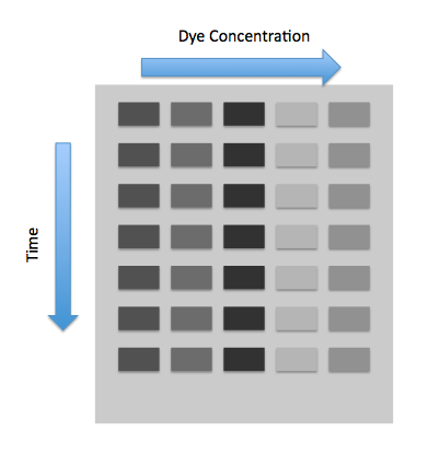
We will also have another row for in vitro measurements. From this row we will graph the fluorescence versus the dye concentration, and the fluorescence will level off at some saturation point. Because the saturation point in vitro will be greater than the saturation point in vivo, we must scale all the fluorescence measurements we find in vivo , which is the importance of $S_r$ and $S_p$.
At this point we will find out the scaling factors $S_r$ and $S_p$. Step 1 is to put samples into the plate reader and take more samples of the same concentration and measure them in vitro. Then, we will measure all the wells at the same time point, and find the saturation fluorescence of the in vitro and the in vivo wells. Dividing the two gives us the $S_r$ and $S_p$.
At each time point we will graph the in vivo fluorescence vs. dye concentrations and find the first dye concentration where saturation occurs. This dye concentration is thus the mRNA/protein total concentration, as we will assume that there will be a 1-1 correspondence of dye and mRNA/protein. We then multiply each by the scaling factor $S_r$ or $S_p$ to get the actual mRNA.
Equilibrium Constants
To check, we can find the fluorescent mRNA concentrations from the mRNA values we obtained in vivo. General first order chemical reactions begin (theoretically):
\begin{equation}\alpha [A] + \beta [B] \leftrightarrow \gamma [AB]\end{equation}where $\alpha$, $\beta$, $\gamma$ are coefficients describing the ratio of molecules of $[A]$ and $[B]$ needed to synthesize $[AB]$. $[A]$, $[B]$, and $[AB]$ are different molecule concentrations. After some time, there will be some equilibrium where some amount of $[A]$ and $[B]$ become $[AB]$. So then, the equation at equilibrium becomes:
\begin{equation}(\alpha[A] - \gamma [AB]) + (\beta[B] - \gamma [AB]) \leftrightarrow \gamma [AB]\label{eq:equi}\end{equation}
We will assume that $\alpha$, $\beta$, and $\gamma$ are all equal to 1. Our $[A]$ will be mRNA/protein and $[B]$ will be the dye concentrations. mRNA dye, which is DFHBI, will be $[D_R]$ and protein dye, which is malachite green (MG), will be $[D_P]$. $[R]_0$ and $[P]_0$ are the initial concentrations of RNA and protein, respectively. Our equations are thus:
\begin{equation}([R]_0 - [R_f]) + ([D_R] - [R_f]) \leftrightarrow ([R_f])\end{equation} \begin{equation}([P]_0 - [P_f]) + ([D_P] - [P_f]) \leftrightarrow ([P_f])\end{equation}
The equilibrium constant for RNA, $K_{D_R}$ is then defined as the product of the reaction product concentrations over the reactant concentrations. We will take the equilibrium constant at equilibrium, so from equation \eqref{eq:equi}, we can determine the equilibrium constant. We will have $[A]_0$ and $[B]_0$ instead of $[A]$ and $[B]$ to signify the initial concentrations of $[A]$ and $[B]$.
\begin{equation}K_{D_R} = \frac{[AB]}{([A]_0 - [AB]) ([B]_0 - [AB])}\end{equation}Now inputting our variables for mRNA expression, once again using $[R]_0$ and $[D_R]_0$ to signify initial concentration of $[R]$ and $[D_R]$:
\begin{equation}K_{D_R} = \frac{[R_f]}{([R]_0 - [R_f])([D_R]_0 - [R_f])} \label{eq:8}\end{equation}
we can solve for $[Rf]$ using a quadratic equation based off of \eqref{eq:8}.
\begin{equation}[R_f]^2 \cdot K_{D_R} - [R_f]\cdot [K_{D_R}([R] + D_R) + 1] + K_{D_R} \cdot [R] \cdot {D_R} = 0\end{equation}
\begin{equation}[R_f] = \frac{[K_{D_R}([R][D_R]) + 1] \pm \sqrt{[K_{D_R}([R][D_R]) + 1]^2 - 4 \cdot (K_{D_R}) \cdot (K_{D_R}[R][D_R])}}{2 \cdot K_{D_R}}\end{equation}We can apply the similar procedure for determining the protein concentration.
Degradation
Degradation occurs for both mRNA and protein. After shutting off production of mRNA/protein, one can measure the degradation coefficient. Some intuition reveals that the amount that is degraded is proportional to the amount of mRNA/protein that is present. We will let $\frac{d[R]_D}{dt}$ be the change in the concentration of RNA, and $\alpha$ be the degradation coefficient determining the fraction of RNA that will be degraded in time.
\begin{equation}\frac{d[R]_D}{dt} = -\alpha \cdot [R]\end{equation}
Protein often has another constant attached to degradation, labeled maturation. Maturation $(a)$ takes into account the time it takes for a protein to mature before fluorescence can actually occur. Maturation is also dependent on the amount of protein available. We will let $\frac{d[P]_D}{dt}$ be the change in the concentration of protein, and $\beta$ be the degradation coefficient determining the fraction of protein that will be degraded in time. In this case, the equation would be
\begin{equation}\frac{d[P]_D}{dt} = -(a + \beta) \cdot [P]\label{eq:12}\end{equation}
However, since the fluorogen activated protein (FAP) takes a small amount of time to fold and to bind to the dye, one can make a reasonable assumption that maturation is 0. So the simplified equation is:
\begin{equation}\frac{d[P]}{dt} = -\beta \cdot [P] \label{eq:13}\end{equation}
Equations \eqref{eq:12} and \eqref{eq:13} can be solved by first order linear differential equation techniques. We will let $[R]_{max}$ and $[P]_{max}$ be the theoretical maximum concentration of RNA and protein (can also be thought of as at equilibrium):
\begin{equation}[R] = [R]_{max}\cdot e^{-\alpha \cdot t}\end{equation} \begin{equation}[P] = [P]_{max}\cdot e^{-\beta \cdot t}\end{equation}
From these equations $\alpha$ and $\beta$ can be determined easily.
mRNA Expression
From the mRNA expression equations, we know that
\begin{equation}\frac{d[R]}{dt} = Ts \cdot [D] - \alpha \cdot [R]\end{equation}
where $Ts$ is the transcriptional efficiency and $\alpha$ is the degradation constant associated with mRNA degradation, $\frac{d[R]}{dt}$ is the change in RNA over time, and $[R]$ is the mRNA concentration or amount.
We see next that this is a first order linear equation, as $Ts$, $[D]$ and $\alpha$ are constants. Rearranging, we get
\begin{equation}\frac{d[R]}{dt} + \alpha \cdot [R] = Ts \cdot [D] \label{eq:e1}\end{equation}
The small integrating factor is thus $e^{\alpha \cdot t}$.
Multiplying the small integrating factor through equation \eqref{eq:e1} (Warning: Math ahead!)
\begin{equation}\frac{d[R]}{dt} \cdot e^{\alpha \cdot t} + \alpha \cdot [R] \cdot e^{\alpha \cdot t} = Ts \cdot [D] \cdot e^{\alpha \cdot t}\end{equation} \begin{equation}\frac{d([R]\cdot e^{\alpha \cdot t})}{dt} = Ts \cdot [D] \cdot e^{\alpha \cdot t}\end{equation} \begin{equation}[R]\cdot e^{\alpha \cdot t} = \int \! Ts \cdot [D] \cdot e^{\alpha \cdot t} \ dt\end{equation} \begin{equation}[R]\cdot e^{\alpha \cdot t} = \frac{Ts \cdot [D]}{\alpha} \cdot e^{\alpha \cdot t} + C \label{eq:e2}\end{equation}At $t = 0$, $[R] = 0$. Plugging into \eqref{eq:e2}, we obtain:
\begin{equation}C = \frac{-Ts \cdot [D]}{\alpha}\end{equation} \begin{equation}[R] \cdot e^{\alpha \cdot t} = \frac{Ts \cdot [D]}{\alpha} \cdot e^{\alpha \cdot t} - \frac{Ts \cdot [D]}{\alpha}\end{equation} \begin{equation}[R] = \frac{Ts \cdot [D]}{\alpha} - \frac{Ts \cdot [D]}{\alpha} \cdot e^{-\alpha \cdot t}\end{equation} \begin{equation}[R] = \frac{Ts \cdot [D]}{\alpha} \cdot (1 - e^{-\alpha \cdot t})\label{eq:eR}\end{equation}$Ts$ is then calculated by
\begin{equation} Ts = \frac{[R] \cdot \alpha}{[D] \cdot (1 - e^{-\alpha \cdot t})}\end{equation}Protein Expression
The protein model is a bit different from the mRNA model due to the fact that the amount of protein depends on the amount of mRNA, which is variable. mRNA is only dependent on $[D]$, which is invariable.
The basic equation looks like:
\begin{equation}\frac{d[P]}{dt} = [R] \cdot Tl - \beta \cdot [P]\end{equation}where $[P]$ is the protein concentration or amount, $[R]$ is still mRNA, $Tl$ is the translational efficiency, and $\beta$ is the degradation constant associated with the protein.
Conveniently, we have already solved for our only hurdle to a first order linear equation, the mRNA amount (from equation \eqref{eq:eR}). We will substitute in for mRNA now:
\begin{equation}\frac{d[P]}{dt} = (1 - e^{-\alpha \cdot t}) \cdot \frac{Ts \cdot [D]}{\alpha} \cdot Tl - \beta \cdot [P]\end{equation}
Now we can solve the first order linear equation:
\begin{equation}\frac{d[P]}{dt} + \beta \cdot [P] = (1 - e^{-\alpha \cdot t}) \cdot \frac{Ts \cdot [D]}{\alpha} \cdot Tl\end{equation}
It can be seen that the integrating factor is $e^{\beta \cdot t}$ :
\begin{equation}\frac{d[P]}{dt} \cdot e^{\beta \cdot t} + \beta \cdot [P] \cdot e^{\beta \cdot t} = e^{\beta \cdot t} \cdot (1 - e^{-\alpha \cdot t}) \cdot \frac{Ts \cdot [D]}{\alpha} \cdot Tl\end{equation} \begin{equation}\frac{d([P] \cdot e^{\beta \cdot t})}{dt} = e^{\beta \cdot t} \cdot (1 - e^{-\alpha \cdot t}) \cdot \frac{Ts \cdot [D]}{\alpha} \cdot Tl\end{equation} \begin{equation}[P]\cdot e^{\beta \cdot t} = \int \! (1 - e^{-\alpha \cdot t}) \cdot \frac{Ts \cdot [D]}{\alpha} \cdot e^{\beta \cdot t} \cdot Tl\ dt\end{equation} \begin{equation}[P]\cdot e^{\beta \cdot t} = Tl \cdot \int \! \frac{Ts \cdot [D]}{\alpha} \cdot e^{\beta \cdot t} \ dt - Tl \cdot \int \!\frac{Ts \cdot [D]}{\alpha} \cdot e^{(-\alpha + \beta) \cdot t} \ dt\end{equation} \begin{equation}[P] \cdot e^{\beta \cdot t} = Tl \cdot \frac{Ts \cdot [D]}{\alpha \cdot \beta} \cdot e^{\beta \cdot t} - Tl \cdot \frac{Ts \cdot [D]}{\alpha \cdot (-\alpha + \beta)} \cdot e^{(-\alpha + \beta) \cdot t} + C \label{eq:34}\end{equation}Now we solve for C. When $t = 0$, $P = 0$ :
\begin{equation}C = -Tl \cdot \frac{Ts \cdot [D]}{\alpha} \cdot (\frac{1}{\beta} - \frac{1}{-\alpha + \beta})\end{equation}Substituting into \eqref{eq:34}, we obtain: \begin{equation}[P] \cdot e^{\beta \cdot t} = Tl \cdot \frac{Ts \cdot [D]}{\alpha \cdot \beta} \cdot e^{\beta \cdot t} - Tl \cdot \frac{Ts \cdot [D]}{\alpha \cdot (-\alpha + \beta)} \cdot e^{(-\alpha + \beta) \cdot t} - Tl \cdot \frac{Ts \cdot [D]}{\alpha} \cdot (\frac{1}{\beta} - \frac{1}{-\alpha + \beta}) \end{equation}
FInally, we solve for Tl. Tl is the translational efficiency, which is the second characteristic we were trying to solve for:
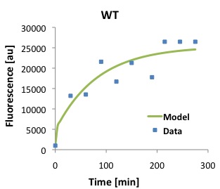
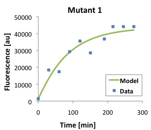
\begin{equation}Tl = \frac{[P]}{\frac{Ts \cdot [D]}{(\alpha \cdot \beta)} \cdot (1 - e^{-\beta \cdot t}) - \frac{Ts \cdot [D]}{\alpha \cdot (-\alpha + \beta)} \cdot (e^{-\alpha \cdot t} - e^{-\beta \cdot t})} \label{eq:Tl}\end{equation}The following figures show that our model described above, and the parameters that we obtained fit well the measured fluorescence for the wild type (WT) promoter and three new promoters (Mutants 1,2, and 3).
Polymerase Per Second
Taking inspiration from ”Measuring the activity of BioBrick promoters using an in vivo reference standard” by Kelly et al.[1], we can derive our own equation for polymerase per second (PoPS), as follows.
mRNA is produced by the number of promoters times the rate of initiations of polymerase onto the promoters, or $n \cdot PoPS$. mRNA is degraded by the degradation equation we derived earlier, which is $-\alpha \cdot [R]$ :
\begin{equation}\frac{d[R]}{dt} = n \cdot PoPS - \alpha \cdot [R] \label{eq:Po1}\end{equation}
where $n$ is the number of promoters in a cell, PoPS is the rate of initiations of RNA polymerase onto the promoters.
Protein is produced by the translational efficiency times the mRNA, which is $[R] \cdot Tl$. Protein is degraded by the degradation equation we derived above, which is $-\beta \cdot [P]$ :
\begin{equation}\frac{d[P]}{dt} = [R] \cdot Tl - \beta \cdot [P] \label{eq:Po2}\end{equation}
At steady state, it can be assumed that $d[R] = 0$ and $d[P] = 0$.
So simplifying \eqref{eq:Po1} and \eqref{eq:Po2}, we obtain:
\begin{equation}PoPS = \frac{\alpha \cdot [R]}{n}\end{equation}Substituting leaves:
\begin{equation}PoPS = \frac{\alpha \cdot \beta \cdot [P]}{n \cdot Tl} \label{eq:PoPS}\end{equation}
The output of the model is polymerase per second, which is what we have found here. It is important to realize that the purpose of finding polymerase per second is that for the current environment of a promoter and the specific type of promoter, it can be characterized using polymerase per second. Experiments can thus easily be conceived by running two experiments on the same promoter under different conditions to see how a promoter is affected, or by running two experiments on different promoters under the same conditions to see which is a stronger promoter.
Fitting
With the data we were given, we decided to fit the equations we derived to the data. We used a method of gradient descent to minimize the error from our fits. We began by trying to fit the transcriptional strength equation, equation \eqref{eq:eR}. We defined our fitting function, $R_i$, in terms of our equation for transcriptional strength, \eqref{eq:eR}, as well as some error $\epsilon$. Since the experimental data was taken in discrete time, we took each point for RNA to be $R_i$ and each point for time to be $t_i$.
\begin{equation}R_i = f(t_i) + \epsilon\end{equation}
\begin{equation}R_i = \frac{T_s}{\alpha} \cdot D \cdot (1 - e^{-\alpha \cdot t_i}) + \epsilon\end{equation}
\begin{equation}R_i = \frac{T_s}{\alpha} \cdot D - \frac{T_s}{\alpha} \cdot D \cdot e^{-\alpha \cdot t_i} + \epsilon\end{equation}
$D$ represents the concentration of DNA, and we are looking for $T_s$ and $\alpha$ as the outputs from our fitting model.We want to minimize our error. To do this, we will use a common method called the method of least squares. We define our error function to be $L(T_s, \alpha)$.
\begin{equation}L(T_s, \alpha) = \sum^n_{i = 1}(R_i - f(t_i))^2\end{equation}
\begin{equation}L(T_s, \alpha) = \sum^n_{i = 1}(R_i - (\frac{T_s}{\alpha} \cdot D - \frac{T_s}{\alpha} \cdot D \cdot e^{-\alpha \cdot t_i}))^2\end{equation}
Now we use a method called gradient descent. This function, over the course of many trials, increments the variables, in our case $T_s$ and $\alpha$, such that the variables gradually approach acceptable values for a fitted function. To do this, we take the derivative of our error function with respect to both our variables, $T_s$ and $\alpha$.
\begin{equation}\frac{\delta L}{\delta T_s} = \sum^n_{i = 1}(2\cdot(R_i - \frac{T_s}{\alpha} \cdot D - \frac{T_s}{\alpha} \cdot D \cdot e^{-\alpha \cdot t_i} \cdot ( -\frac{D}{\alpha} + \frac{D}{\alpha} \cdot e^{\alpha \cdot t_i})))\end{equation}
\begin{equation} \begin{split}\frac{\delta L}{\delta \alpha} &= \sum^n_{i = 1}(2 \cdot (R_i - \frac{T_s}{\alpha} \cdot D + \frac{T_s}{\alpha}\cdot D \cdot e^{-\alpha \cdot t_i})\cdot \\&(\frac{T_s \cdot D}{\alpha^2} - \frac{T_s \cdot D}{\alpha^2} \cdot e^{-\alpha \cdot t_i} + \frac{T_s}{\alpha} \cdot D \cdot e^{-\alpha \cdot t_i}\cdot (-t_i)))\end{split}\end{equation}
From here, we begin incrementing $T_s$ and $\alpha$ for a number of trials $K$.
\begin{equation}T^{k + 1}_s = T^k_s + \eta \cdot \frac{\delta L}{\delta T^k_s}\end{equation} for k = 1... K.
$\eta$ is a term often called "learning rate" in machine learning, but which we will call step size. It is called thusly due to the fact that $T_s$ and $\alpha$ are incrementing a different amount every time based on the closeness of the fit for each trial. In this sense, the variables could be seen as "learning" where the optimal fitting values are and changing their increments accordingly. $\eta$ is equivalent to the inverse of the number of trials, K. $\eta = \frac{1}{K}$.
We can do a similar equation for $\alpha^{k + 1}$.
\begin{equation}\alpha^{k + 1} = \alpha^k + \eta \cdot \frac{\delta L}{\delta \alpha ^k}\end{equation} for k = 1...K.
The final values, $T^K_s$ and $\alpha^K$ are the parameters we are looking for in our fitting function.
For our translational efficiency model, we performed the same set of methods to get our fit. We will use our fitted variables from the transcriptional strength fitting in our translational efficiency fitting so that we still are only fitting 2 variables. We first defined our fitting function, $M(Tl, \beta)$.
\begin{equation}\begin{split}[P] &= Tl \cdot \frac{T_s \cdot D}{\alpha \cdot \beta} - Tl \cdot \frac{T_s \cdot D}{\alpha \cdot (-\alpha + \beta)} \cdot e^{-\alpha \cdot t} - Tl \cdot \frac{T_s \cdot D}{\alpha \cdot \beta} \cdot e^{-\beta \cdot t} \\&+ Tl \cdot \frac{T_s \cdot D}{\alpha \cdot (-\alpha + \beta)} \cdot e^{-\beta \cdot t} + \epsilon \end{split}\end{equation}
\begin{equation}[P] = Tl \cdot (\frac{T_s \cdot D}{\alpha}\cdot (\frac{1}{\beta}\cdot (1 - e^{-\beta \cdot t}) - \frac{1}{-\alpha + \beta}(e^{-\alpha \cdot t} - e^{-\beta \cdot t}))) + \epsilon\end{equation}
\begin{equation} M(Tl, \beta) =\sum^n_{i = 1}([P] - Tl \cdot (\frac{T_s \cdot D}{\alpha}\cdot (\frac{1}{\beta}\cdot (1 - e^{-\beta \cdot t}) - \frac{1}{-\alpha + \beta}(e^{-\alpha \cdot t} - e^{-\beta \cdot t}))))^2\end{equation}
Again, we take the partial derivatives with respect to each variable, in our case $Tl$ and $\beta$.
\begin{equation} \begin{split} \frac{\delta M}{\delta Tl} &= \sum^n_{i = 1}(2([P] - Tl \cdot (\frac{T_s \cdot D}{\alpha}\cdot (\frac{1}{\beta}\cdot (1 - e^{-\beta \cdot t}) - \frac{1}{-\alpha + \beta}(e^{-\alpha \cdot t} - e^{-\beta \cdot t})))) \cdot (\frac{T_s \cdot D}{\alpha})\\ &\cdot (\frac{1}{\beta}\cdot (1 - e^{-\beta \cdot t}) - \frac{1}{-\alpha + \beta} \cdot e^{-\beta \cdot t}))\end{split} \end{equation}
\begin{equation} \begin{split} \frac{\delta M}{\delta \beta} &= \sum^n_{i = 1}(2([P] - Tl \cdot (\frac{T_s \cdot D}{\alpha}\cdot (\frac{1}{\beta}\cdot (1 - e^{-\beta \cdot t}) - \frac{1}{-\alpha + \beta}(e^{-\alpha \cdot t} - e^{-\beta \cdot t})))) \cdot \\&(Tl \cdot \frac{T_s \cdot D}{\alpha} \cdot (\frac{-1}{\beta^2}\cdot (1 - e^{-\beta \cdot t}) + \frac{t \cdot e^{-\beta \cdot t}}{\beta} + \frac{1}{(-\alpha + \beta)^2} \cdot (e^{-\alpha \cdot t} - e^{-\beta \cdot t}) - \frac{1}{-\alpha + \beta}\cdot(t \cdot e^{-\beta \cdot t}))))\end{split}\end{equation}
We will increment $Tl$ and $\beta$ similar to the $T_s$ and $\alpha$ incrementing, with $K$ being the number of trials and $\eta$ being the step size.
\begin{equation}Tl^{k + 1} = Tl^k + \eta \cdot \frac{\delta M}{\delta Tl^k}\end{equation} for k = 1...K.
\begin{equation}\beta^{k + 1} = \beta^k + \eta \cdot \frac{\delta L}{\delta \beta^k} \end{equation} for k = 1...K.
As a summary, we can minimize the error of the fitting using the above techniques. This algorithm for minimizing error can be best utilized in code, due to the fact that an accurate fit requires a large $K$.
[1] Kelly, Jason R., Adam J. Rubin, Joseph H. Davis, Caroline M. Ajo-Franklin, John Cumbers, Michael J. Czar, Kim De Mora, Aaron L. Glieberman, Dileep D. Monie, and Drew Endy. "Measuring the Activity of BioBrick Promoters Using an in Vivo Reference Standard." Journal of Biological Engineering 3.1 (2009): 4. Print.